Asymptotics of the Solution to a Stationary Piecewise-Smooth Reaction-Diffusion-Advection Equation∗

Qian YANG Mingkang NI

Abstract A singularly perturbed boundary value problem for a piecewise-smooth nonlinear stationary equation of reaction-diffusion-advection type is studied.A new class of problems in the case when the discontinuous curve which separates the domain is monotone with respect to the time variable is considered.The existence of a smooth solution with an internal layer appearing in the neighborhood of some point on the discontinuous curve is studied.An efficient algorithm for constructing the point itself and an asymptotic representation of arbitrary-order accuracy to the solution is proposed.For sufficiently small parameter values,the existence theorem is proved by the technique of matching asymptotic expansions.An example is given to show the effectiveness of their method.

Keywords Reaction-Diffusion-Advection equation, Internal layer, Asymptotic method, Piecewise-Smooth dynamical system

1 Introduction

In recent years, reaction-diffusion-advection equation with a small parameter that is also called singularly perturbed equation has attracted much attention due to their practical use as mathematical models in optical electronics, medical science, in-situ combustion problems,atmospheric science, etc (see [1–4]).Generally speaking, this kind of problem is studied by several methods such as geometric singular perturbation theory(see[5–10]),asymptotic method(see [11–15]), numerical algorithm (see [16–19]).

This paper investigates a boundary value problem for a stationary case of piecewise-smooth reaction-diffusion-advection equation.In this case,the nonlinear function on the right of differential equation is discontinuous on some monotone discontinuity curve.The main complexity of this problem is the existence of a smooth solution with a steep gradient in the neighborhood of some point on this curve, which is called the internal layer (see [20–26]).The biggest challenge is to determine the transition point itself and an asymptotic approximation of the smooth solution.Similarly stated problems have been considered in [27–35].As studied in papers [30–35],the discontinuity line located in the domain of function on the right of differential equation is vertical to the time variable.Using a new method, we shall generalize the basic results in the case of problems with discontinuous time variables(see[35])to the case of equations whose state variables are discontinuous.Moreover, our results can be used to develop efficient numerical algorithms for some models with discontinuous coefficients (see [36–37]).

1.1 Model problem

We will consider the singularly perturbed boundary value problem

whereµ>0 is a small parameter, anduis an unknown scalar function.

Let

It is easy to see that problem(1.1)is equivalent to the following system of first-order differential equations:

Suppose that the following conditions are satisfied.

Condition 1The functionf(v,u,x) has the form

where

here functionsf(∓)(v,u,x) are sufficiently smooth on the sets {v| −l1≤v≤l1} ×D(∓).Moreover,g(x) is sufficiently smooth and monotonely nondecreasing in the interval 0 ≤x≤1.As shown in Figure 1, the discontinuous curve Γ :u=g(x),0 ≤x≤1 separates the domainD={(u,x)|−l≤u≤l,0 ≤x≤1} into two subdomainsD(∓).

Condition 2Assume that the degenerate equationf(∓)(0,u,x) = 0 has isolated rootsu=ϕ(∓)(x) on the subdomainsD(∓), and one has the inequalities:

(a)f(−)(0,g(x),x)≠f(+)(0,g(x),x),0 ≤x≤1,

(b)(0,ϕ(∓)(x),x)>0,(ϕ(∓)(x),x)∈D(∓).

As shown in Figure 1, two curvesy=ϕ(−)(x) andy=ϕ(+)(x) intersect the curvey=g(x)at two pointsQandP, whose abscissas are denoted byqandp, respectively, in thexyplane.Ifp < q, then problem (1.1) may have a solution with a sharp internal layer in the neighborhood ofx=x∗(0< x∗<1).The transition pointx∗where the solution passes through the monotone curve is unknown beforehand.Similarly, the case when the functiong(x) is monotonely nonincreasing in the interval [0,1] can also be considered.

Figure 1 The solution of problem (1.1).

Figure 2 Graphic illustration of the separatrix Φ(,x)=Φ(0,ϕ(−)(x∗),x∗) issuing from the saddle point (ϕ(−)(x∗),0) and the separatrix Φ(,x)=Φ(0,ϕ(+)(x∗),x∗) entering the saddle point(ϕ(+)(x∗),0).

Figure 3 Graphic illustration of the heteroclinic orbit between saddle points (ϕ(−)(x∗),0) and(ϕ(+)(x∗),0).

1.2 Associated system

Consider the associated system (see [11]),

where∈[0,1] is a parameter.

By virtue of Conditions 1–2, the characteristic equation

has two roots of different signs.The reason behind this is that

The associated system (1.3) defines equations

for the phase trajectories on the planefor any∈[0,1].

Condition 3Suppose that the separatrices which are described by (1.4) with the initial conditions

By Conditions 1–3, in the plane, for any fixed, there exist separatrixespassing through the saddle points (ϕ(∓)(),0).In the course of determining the leading terms in the asymptotic expansion of boundary layer,the solvability of the following boundary value problems for system (1.3) taken atplays an important role:

and

According to Conditions 1–3,in the phase plane,there exists a stable manifoldΦ(0,ϕ(−)(0),0) passing through the saddle point (ϕ(−)(0),0), and there exists a stable manifoldpassing through the saddle point (ϕ(+)(1),0).Therefore, if boundary valuesu0andu1are located on the corresponding stable manifolds, then problems(1.6) and (1.7) are solvable.

Condition 4Suppose that in the phase planethe vertical lineintersects the stable manifoldpassing through the saddle point (ϕ(−)(0),0),and the vertical line=u1intersects the stable manifoldpassing through the saddle point (ϕ(+)(1),0).

To determine the leading term in the asymptotic expansion of internal layer,it is necessary to consider the following boundary value problem for system (1.3) taken atx=x∗:

whereg(x∗) ∈[ϕ(+)(x∗),ϕ(−)(x∗)].Then in the phase plane, there are two separatrixes in and out passing through each of saddle points (ϕ(∓)(x∗),0).Without loss of generality, we assume that these separatrixes lie in the lower half-plane<0.Thus, one can obtain the following sufficient condition needed to guarantee that problem (1.8) is solvable.

Condition 5Suppose that the separatrixissuing from the saddle point (ϕ(−)(x∗),0) intersects the vertical liney=g(x∗), and the separatrixΦ(0,ϕ(+)(x∗),x∗) entering the saddle point (ϕ(+)(x∗),0) intersects the vertical liney=g(x∗)in the phase plane(see Figure 2).

As shown in Figure 1, the transition pointx∗where the solution of problem(1.1)passes the monotone curve is unknown.To findx∗, for anyx∈[p,q], we introduce the function

Condition 6Assume that the equation H(x) = 0 has a solutionx=x0,x0∈[p,q] (see Figure 3), and the inequality H′(x)(x0)≠0 holds.

2 Formal Asymptotics

As shown in Figure 1, problem (1.1) may have a solution with an internal transition layer in the neighborhood of monotone curvey=g(x).To construct an asymptotic approximation to the solution of problem(1.1)that has an internal layer separately on the intervals[0,x∗]and[x∗,1], we consider two classical boundary value problems

Then we match the asymptotic expansions of the solutions to problems(2.1), (2.2)at the transition point (x∗,g(x∗)) smoothly.Thus, a smooth asymptotic solution of the original problem(1.1) with an internal layer in the neighborhood of discontinuous curvey=g(x) is obtained.To this end, it is necessary to satisfy the following smoothness condition

where the unknown point (x∗,g(x∗)) shall be found by the matching asymptotic expansion method after constructing the asymptotics of solutions to problems (2.1), (2.2).

In order to describe the solution in a sharp internal layer region and in the neighborhood of endpoints of the interval [0,1], the stretched variables are introduced:

Note that the solution in region without steep gradient depends on the slow variablex.Then we write out the asymptotic representations of two auxiliary problems (2.1), (2.2):

Each function of asymptotic representations (2.4), (2.5) shall be written in the forms of power series of small parameterµ:

where(τ)(τ), Lku(τ0), Lkv(τ0), Rku(τ1), Rkv(τ1) (k≥0) are imposed the standard conditions at infinity:

In order to determine high-order asymptotic terms of internal layer and boundary layerandLku(τ0), Lkv(τ0), Rku(τ1), Rkv(τ1) (k≥1), the following condition is also needed.

Condition 7Suppose that one has the inequalities

2.1 Regular part

The equations for determining the regular termstake the form

Substituting (2.6)–(2.7)into (2.16)and matching the coefficients of like powers ofµ, we obtain the degenerate equations

whose solution are

by Condition 2.

By virtue of Condition 2, the remaining coefficientsare obtained by linear equations

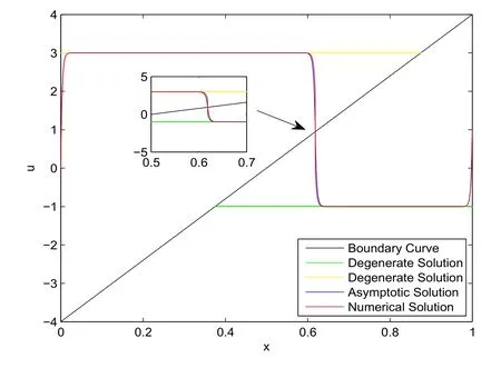
where(x)is known functions that depends on(x)(j

In particular,

2.2 Internal layer functions

The problems for finding the internal layer functionsQ(∓)u(τ), Q(∓)v(τ) at the transition point (x∗,g(x∗)) are as follows

After substituting (2.12)–(2.13) into (2.17) and matching the coefficients of like powers of µ,one can obtain the problems for determining

By means of variable substitution

problem(2.18)can be rewritten as(1.8).According to the discussion of associated system(1.8),problem (2.18) has solutionswhich satisfy the exponential estimates (see[11])

where

The equations of problem (2.21) can be rewritten as second-order differential equations

Thus, one can obtain the Cauchy problem

whose solutions can be represented in the forms

where

From (2.23) and (2.25), functions(τ),(τ) have the exponential estimates of the type (2.20).

2.3 Boundary layer terms

The equations and boundary value conditions for determining left boundary layer functionsLu(τ0), Lv(τ0) at the endpointx=0 have the forms

Likewise, the problems for finding the right boundary layer functionsRu(τ1), Rv(τ1) at the endpointx=1 can be obtained

ForL0u(τ0), L0v(τ0) andR0u(τ1), R0v(τ1), we have

Considering the discussions about auxiliary systems(1.6)and(1.7),problems(2.28)and (2.29)have solutionsL0u(τ0), L0v(τ0)andR0u(τ1), R0v(τ1)accordingly.In addition,if Conditions 1–4 are satisfied,then functionsL0u(τ0), L0v(τ0)andR0u(τ1), R0v(τ1)have exponential estimates of type (2.20).

The problems for determiningLku(τ0), Lkv(τ0) andRku(τ1), Rkv(τ1) have the forms

By Condition 7, the solutions of problems (2.30) and (2.31) can be represented as

It follows from(2.32)–(2.35)thatLku(τ0), Lkv(τ0)andRku(τ1), Rkv(τ1) also satisfy the exponential estimates similar to (2.20).

3 Existence of a Smooth Solution to the Original Problem (1.1)

Suppose thatx∗exists, then solutions of two auxiliary problems (2.1) and (2.2) are defined in the regions[0,x∗]×[g(x∗),l]and [x∗,1]×[−l,g(x∗)] respectively.Thus, it is easy to see that these two problems are classical singularly perturbed two point boundary value problems whose asymptotic solutions are smooth on both sides of monotone curvey=g(x).In the following,the existence ofx∗is proved and we justify the fact that composite solution obtained in Section 2 is smooth at the transition point (x∗,g(x∗)).

We representx∗in the form of the sum

whereδis a parameter.

As proved in [11], problems (2.1), (2.2) have solutionsu(∓)(x,µ,δ), whose asymptotic representations are

here the internal layer functions(τ)(τ) depend onand the unknown parameterx∗.Taking account ofand expanding both sides of the smoothness condition (2.3) into power series ofµ, one can obtain the matching conditions that make sure the asymptotic solution is smooth at the point (x∗,g(x∗)):

where(x0,···,xk−1) are known functions depending onx0,···,xk−1.By virtue of Condition 6, there existsx0∈(p,q) such that H(x0) = 0, thus, (3.3) is satisfied, and (3.3) can be rewritten asTherefore, the leading term ofx∗is found.Below we will discuss how to findx1.

Lemma 3.1Under Condition6, x1is determined by the linear equation

ProofTakinginto consideration, and substituting (2.23), (2.25) into(3.4), we have

which can be simplified as

by using the equality

In order to make sure that the coefficient ofx1in the linear equation above is nonzero, it is necessary to obtain the representation of H′(x0).

Let

Differentiating with respect toxfor the equations of problem (1.8), we have

Applying Green formula leads to

By virtue of Condition 5, the separatrixesdo not intersect=0 asτ= 0.Thus,(0) ≠ 0.Therefore, (3.6) can be rewritten as (3.5).By Condition 6,x1can be uniquely determined by the linear equation (3.5).

Similarly,xk(k=2,3,···) can be obtained by the same algorithm.

Denote

Substituting the asymptotic representations (3.2) ofu(∓)(xδ,µ) intoG(xδ,µ), it follows from H(x0)=0, Lemma 3.1 and the algorithm of constructingxk(k≥2) that

By Condition 6, H′(x0)≠0, for sufficiently smallµ, there existsδ=such thatG()=0.Thus, providedδ=in the representation (3.1), the obtainedwill guarantee that the composite function

is a smooth contrast structure solution to problem (1.1) in the neighborhood ofx=.After replacingby, the accuracy of the first equation of (3.2) remains constant.So the main theorem in this paper can be derived.

Theorem 3.1Under Conditions1–7, for sufficiently small µ>0, the nonlinear boundary value problem(1.1)has a smooth contrast structure solution u(x,µ), whose asymptotic representations are as follows

and an internal layer appears in the neighborhood of the discontinuous curve y=g(x).

4 Example

We consider the second order nonlinear Dirichlet boundary value problem

whereg(x)=8x−4.

Since the reaction-diffusion-advection equation with a small parameter is an important mathematical model in different research fields, this example has a profound practical background.Example (4.1) can be used to develop mathematical models in mechanics, electronics,biology, and other fields in the case when phenomena in inhomogeneous media with discontinuous characteristics occur.In [1], a multidimensional singularly perturbed reaction-diffusionadvection problem with wave functions of electrons and holes and Coulomb potential depending on the parameters of the layer is studied and the increase of tunnel barrier transparency leads to a transition from the dipolar electron-hole system (EHS for short) with a double-peak wave function of electrons to the spatially direct EHS.Furthermore,to describe an in-situ combustion process,the reaction-diffusion-advection mathematical model with an internal layer is proposed in [3].Based on our theoretical results, the asymptotic behavior of a solution to example (4.1)shall be discussed.

Letµ=0, we haveϕ(−)(x)=3,ϕ(+)(x)=−1 and

It is easy to verify that Conditions 1–7 in Theorem 3.1 are satisfied.The function (1.9)can be rewritten as

and the equation H(x0)=0 has a solutionx0=0.6204.The computation shows that H′(x0)≠0, so Condition 6 is also satisfied.

The problems for determininghave the forms

whose solutions are

ForL0u, R0u, we have

and

whose solutions acquire the forms

From the linear equation (3.5), one can obtainx1=0.6429.

Applying Theorem 3.1, problem (4.1) has a smooth asymptotic solutionu(x,µ), which can be represented as

where

This problem has not an analytical solution,whose behavior can be described by an asymptotic solution obtained by our method.In addition, asµtakes sufficiently small value, the accuracyO(µ) of the obtained smooth asymptotic solutiony(x,µ) is very small.As shown in Figure 4, our asymptotic solution is close to the numerical solution and there is an internal layer in the neighborhood of discontinuous curvey=8x−4.

Figure 4 Numerical solution of problem (4.1) and its zero-order asymptotic approximation(µ=0.003).

5 Conclusion

This paper investigates a stationary problem for a reactive-advection-diffusion differential equation with discontinuous right-hand side.The sufficient conditions for the existence of a smooth solution with an internal layer in the neighborhood of a point on the discontinuous curve is given.Using theorems on existence of solutions to classical boundary value problems for singularly perturbed nonlinear equations and algorithm for constructing asymptotic expansions to these solutions, the existence of a smooth solution is proved.This work is an extension and further development of the results in [35].What’s more, our method can be generalized to multidimensional singularly perturbed reaction-diffusion-advection problems.The results can also be applied to propose an efficient numerical algorithm that uses the asymptotic solution to construct non-uniform meshes to describe the behavior of internal layer of the solution to similar problems stated in [36–37].

AcknowledgementThe authors would like to express their deepest gratitude to the anonymous reviewers for their careful work, valuable comments and thoughtful suggestions.