High‑accuracy measurement of Compton scattering in germanium for dark matter searches
2023-01-05HaiTaoJiaShinTedLinShuKuiLiuHsinChangChiMuhammedDenizChangHaoFangPengGuXiJiangYiKeShuQianYunLiYuLiuRenMingJieLiChenKaiQiaoChangJianTangHenryTszKingWongHaoYangXingLiTaoYangQianYueYuLuYanKangKangZhaoJ
Hai‑Tao Jia · Shin‑Ted Lin · Shu‑Kui Liu · Hsin‑Chang Chi · Muhammed Deniz · Chang‑Hao Fang ·Peng Gu · Xi Jiang · Yi‑Ke Shu · Qian‑Yun Li · Yu Liu · Ren‑Ming‑Jie Li · Chen‑Kai Qiao · Chang‑Jian Tang ·Henry Tsz‑King Wong · Hao‑Yang Xing · Li‑Tao Yang · Qian Yue · Yu‑Lu Yan · Kang‑Kang Zhao ·Jing‑Jun Zhu
Abstract Compton scattering with bound electrons contributes to a significant atomic effect in low-momentum transfer, yielding background structures in direct light dark matter searches as well as low-energy rare event experiments. We report the measurement of Compton scattering in low-momentum transfer by implementing a 10-g germanium detector bombarded by a 137Cs source with a radioactivity of 8.7 mCi and a scatter photon captured by a cylindrical NaI(Tl) detector. A fully relativistic impulse approximation combined with multi-configuration Dirac—Fock wavefunctions was evaluated, and the scattering function of Geant4 software was replaced by our calculation results. Our measurements show that the Livermore model with the modified scattering function in Geant4 is in good agreement with the experimental data. It is also revealed that atomic many-body effects significantly influence Compton scattering for low-momentum transfer (sub-keV energy transfer).
Keywords Compton scattering experiment · Germanium detector · Atomic many-body effects · Geant4 · Dark matter
1 Introduction
There is overwhelming evidence from astronomy [1—4],astrophysics, and cosmology [5—7] that dark matter (DM)may be the dominant form of matter in the universe, and weakly interacting massive particles (WIMPs) are widely regarded as the most attractive and promising candidates[8]. The null results of WIMP DM searches from direct DM detection experiments, such as Xenon [9], PandaX [10],CDEX [11—13], DarkSide [14], SuperCDMS [15], and other experiments [16—19], have motivated a comprehensive survey on the mass range and a diverse search of non-WIMP DM models, such as axion-like particles, dark photon particles, millicharged particles, and the interaction of DM with electrons [20—24].
Searches of low-mass WIMPs and several DM models require dedicated low-threshold detector technologies and ultralow-background environments [25—27]. High-purity germanium (HPGe) and liquid xenon are widely used in the direct detection of DM [28—31]. However, the interpretation of DM experimental data depends on a better background understanding of the low-energy region. The capability of detector technologies to differentiate nuclear recoils from electronic recoils is generically suppressed near the threshold, whereas some technologies are indistinguishable in both types of recoils. Background from Compton scattering via gamma rays from radioactive materials is invertible in terrestrial detectors aimed at direct-detection DM searches. In particular, Compton scattering with low-momentum transfer is critically involved in atomic many-body effects [32—34].Therefore, a precise measurement and an atomic many-body calculation of Compton scattering are essential not only for background understanding but also for the detection channel for the identification of DM. In addition, understanding the Compton scattering process would facilitate other areas of research, such as laser electron gamma sources and Compton cameras [35—38].
To obtain a comprehensive understanding of the Compton scattering process in detectors, a combined study of experimental measurements and Monte Carlo simulations was conducted. Herein, we focus on Compton scattering in HPGe detectors and the small-angle Compton scattering process, which corresponds to low-energy and low-momentum transfer cases.
In the conventional Monte Carlo simulation program Geant4, Compton scattering is used for free electron approximation (FEA) or impulse approximation (IA) [39—44].However, in the Geant4 program, several old databases containing Compton scattering results calculated by Biggs and Hubbell et al. are adopted for various simulation models[45—47], and these databases are insufficient and incapable of providing precise predictions. First, they calculated the incoherent scattering function (SF) and Compton profile using nonrelativistic Waller—Hartree (WH) formalism and Hartree—Fock (HF) wavefunctions. Second, in the conventional HF, which is a single-configuration formalism, atomic many-body effects are inadequate. Therefore, improved databases that consider relativistic and many-body effects are needed.
In this study, we analyzed several simulation models in the Geant4 program and improved these models by replacing the old nonrelativistic atomic databases with our ab initio calculations. Our calculations were implemented using fully relativistic multi-configuration Dirac—Fock (MCDF)wavefunctions [48]. With an efficient algorithm for handling many-body effects (such as electron correlations,electron exchanges, and atomic configuration interactions)and relativistic effects, the MCDF formalism provided more accurate databases for atomic and molecular processes. For small-angle Compton scattering, there were clear differences between our results and those of conventional Geant4 simulations.
A high-accuracy Compton scattering experiment was designed and conducted to test the validity of the new simulation results. HPGe was chosen as the prime detector, and sodium iodide (NaI) acted as the coincidence detector. Each Compton event in the experiment was identified using coincidence detection. The least squares method was adopted for data analysis. The differential cross sections and incoherent SF in the Compton scattering process were accurately measured in our experiments and carefully compared with the simulation predictions. In particular, we mainly analyzed the results for small scattering angles, where the energy and momentum transfer in Compton scattering were small.
The remainder of this paper is organized as follows:Sect. 2 provides a description of the theoretical framework, Sect. 3 focuses on the experimental design, Sect. 4 is devoted to data analysis, and Sect. 5 presents the experimental results. A summary is presented in Sect. 6.
2 Theoretical framework and Monte Carlo simulation
2.1 Compton scattering in the framework of free electron approximation and relativistic impulse approximation
whereθis the scattering angle,mis the electron mass, andcis the speed of light. In FEA, the differential cross section is determined using the Klein—Nishina formula [40]

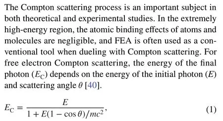
wherer0is the classical electron radius. This formula describes the case of free electron scattering without considering the atomic binding effects and pre-collision motions of the target electrons. However, in certain circumstances,the pre-collision motion has a large influence, known as the Compton peak [49, 50], on the dispositional energy spectrum, as shown in Fig. 1.
Atomic binding and Doppler broadening effects are largely incorporated into relativistic impulse approximation(RIA) [41—44]. From RIA, the Compton scattering cross section can be accurately calculated. In RIA, a doubly differential cross section (DDCS) is factorized into a kinematical factor and momentum-dependent function. In this framework, the DDCS of the Compton scattering process between electrons and unpolarized incident photons can be expressed as [43]
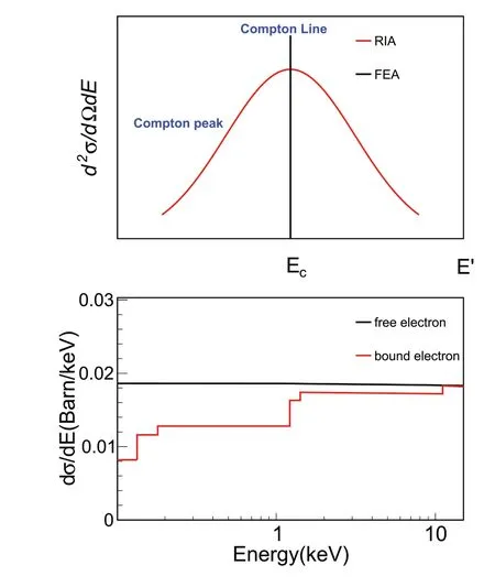
Fig. 1 Compton energy spectrum with bounded electrons versus free electrons

whereE′is the energy of the scattered photon,qis the modulus of the momentum transfer vector q=k −k′, k and k′are the momentum of the incident and scattered photons, respectively,pzis the projection of the electron momentum in the momentum transfer direction, the factorX(R,R′) in Eq. (3)was defined by Ribberfors [39, 43], andZiis the number of electrons inith subshell. The momentum-dependent functionJi(pz) is the Compton profile in this subshell [39, 43, 44]

whereρi(pz) is the electron momentum distribution in theith subshell, which can be obtained from ground-state wavefunctions. The step function Θ(E−E′−Ui) accounts for the electron taking part in Compton scattering, which is activated only if the transferred energyE−E′is larger than the atomic binding energy of theith subshellUi.
The single-differential cross section (SDCS) of Compton scattering can be obtained by integrating the DDCS over the allowed scattered energies. Under certain approximations of the functionX(R,R′) , this can be written as [43, 44, 51]


In fact,xdepends on the momentum transfer in the scattering process.
2.2 Multi‑configuration Dirac–Fock method results on the Compton profile and scattering function
In the theoretical calculation and Monte Carlo simulation of Compton scattering, the atomic Compton profileJ(pz) and incoherent SF are obtained by integrating the momentum distributions of the electrons. To acquire this momentum distribution and ground-state wavefunction Ψ , an MCDF approach can be implemented [48, 52].
The MCDF approach is a generalization of the Dirac—Fock or HF method and is more efficient for describing atomic and molecular states. In the MCDF formalism,more electron correlations and configuration interactions are included. In this formalism, the many-body groundstate wavefunction Ψ is a superposition of the configuration wavefunctionψa,

and the configuration wavefunctionψacan be constructed from the Slater determinant of Dirac orbitals.Caandψain the MCDF wavefunction Ψ are determined from the variational principle.
In this study, we adopted a two-configuration groundstate wavefunction for germanium,

where the symbol (nl2j)0denotes the Slater determinant constructed from twonljvalence orbitals and all core orbitals with a total angular momentumJ=0 and even parity. For germanium, the theoretical MCDF binding energies, binding energies from the Geant4 databases, and experimental edge energies [53—57] are listed in Table 1.
In the simulation program Geant4, the tabulated Compton profile given by Biggs et al. [46] is calculated within nonrelativistic HF wavefunctions, and incoherent SFs are obtained by fitting the data from the EPDL databases provided by Hubbell et al. [45, 47], whose calculations are within nonrelativistic WH theory and HF wavefunctions [58]. In these old databases, atomic relativistic effects and some electron correlation effects were not considered.
In this study, to obtain a more accurate prediction, we improved these databases using ab initio calculations. We calculated the Compton profile and incoherent SF using fully relativistic MCDF wavefunctions with atomic relativistic effects, electron correlations, and configuration interactions.The discrepancies in the incoherent SFs between our calculations and the Geant4 databases are shown in Fig. 10. It is clear that the differences in SF are explicit in low-momentum transfer cases (with smallx).
2.3 Monte Carlo simulation models

Fig. 2 (Color online) Upper figure shows the SDCS of the three models. The lower figure shows the energy spectrum generated by the three models when the scattering angle is 5 ◦ . The incident photon energy is 662 keV
In this study, the Geant4 program (10.05 version) was used for Monte Carlo simulations. There are three models in the Geant4 program when simulating Compton scattering in the low-energy region: the LivermoreComptonModel, LowEPComptonModel (Monash Model), and PenelopeModel. The simulation results based on the three models are shown in Fig. 2. It is clear that the SDCSs of the three models were similar. However, there were notable differences between the DDCSs of these models. Both the Livermore and Penelope models treat the collision of photons and electrons in a twodimensional scattering plane [59]; therefore, the difference between these two models was very small. Under these circumstances, we chose the Livermore model among the two models (Penelope and Livermore) as a representative model. The Monash model uses a two-body complete relativistic three-dimensional scattering framework to ensure that energy and momentum are conserved in RIA [60].Compared with the Livermore and Penelope models, the DDCS in the Monash model was different. In this study,we conducted an experiment to test the simulation results of the Livermore and Monash models. Furthermore, the experimental ionization energy of germanium atoms and our ab initio calculation of the Compton profile and the incoherent SF were adopted in the simulation.

Table 1 Theoretical binding energies of germanium atoms calculated using the MCDF formalism, the binding energies of germanium atoms in Geant4 databases, and the experimental edge energies extracted from the photo-absorption data of germanium solids
3 Experimental setup
In this study, an elaborately designed Compton scattering experiment with high precision was performed. This experiment could not only test the theoretical and simulation results but also help us better understand the background of Compton scattering in HPGe in rare-event experiments.
3.1 Experimental design and apparatus
The schematic of the experimental setup depicted in Fig. 3 includes the main HPGe detector, NaI(TI) coincidence detector, and a137Cs gamma source (8.7 mCi).
The HPGe was a 10-g n-type germanium detector with a diameter of 16 mm and a height of 10 mm. A crystal was encapsulated within a cryostat composed of oxygen-free high-conductivity (OFHC) copper. The end cap of the cryostat was composed of carbon composite with a thickness of 0.6 mm, allowing calibration with low-energy gammas outside.
The NaI(Tl) detector, with a threshold of approximately 150 keV, had dimensions of 76 mm in diameter and 120 mm in height. A hole with a diameter of 10 mm and a depth of 50 mm was opened in front of the NaI(Tl) crystal, which improved the detection efficiency of incoming photons along the axial direction of the hole. To reduce the accidental background, the NaI(Tl) detector was surrounded by 5 cm-thick lead, except for a hole with a diameter of 18 mm in front of the detector.
3.2 Experimental angle calibration
In the experiment, the steps below were followed for angle calibration.

Fig. 3 The Schematic diagram of experimental design and apparatus
A horizontal plane was calibrated parallel to the ground using a horizontal leveling laser meter with three laser planes. The precision of the leveling meter was ± 0.3 mm/m,which was equal to 0.1◦in the case of our experiment. Then,all detectors were placed on this calibrated horizontal plane.
Next, a scattering angle of 0◦was determined, that is,the direction of the photons directly emitted by137Cs . The calibration was performed using a small cubic NaI detector with a side length of 6 mm. This small detector was placed atX=1.499 m andX=1.991 m on the calibrated horizontal plane and then moved along theYdirection to obtain the position distributions of the 662 keV peak count rates along theYdirection (in the inset of Fig. 3, the red line representsX=1.991 m and blue line representsX=1.499 m. The centers of the blue and red lines were connected to derive an angle of 0◦.
Subsequently, the arbitrary angle between the germanium detector and the NaI detector was determined. The germanium detector was always fixed at an angle of 0◦,X=25.2 cm, during the entire experiment. Two laser leveling meters were used: the first pointing in the 0◦direction, and the second pointing in an arbitrary direction. The intersection of the two emitted laser beams was set at the center of the germanium detector. The center of the NaI detector was placed in an arbitrary direction and the axial direction of the detector was set along the angle direction according to the second laser beam indication. The NaI detector should be placed as far from the germanium detector as possible to reduce the systematic error on the angle. Within the constraints of the experimental site, the NaI detector was placed 2 m from the germanium detector. In the calculation of the arbitrary angle,the vertical projection coordinates of each detector on the calibrated horizontal plane were measured, and then the side lengths of the triangle formed by the germanium detector,NaI detector, and 0◦direction were calculated according to the coordinates to calculate the value of the scattering angle.
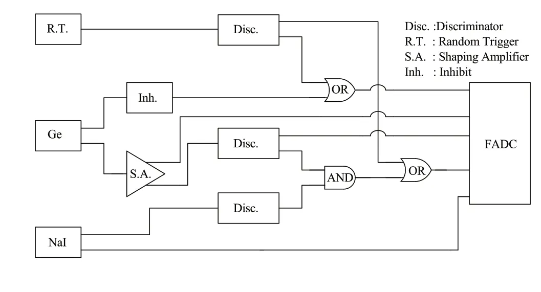
Fig. 4 The electronic schematic of experiment
3.3 Data acquisition (DAQ) system
A schematic of the electronics and data acquisition (DAQ)system is shown in Fig. 4.
The p+ contact signal was read out by a low-noise FET in the vicinity of the germanium crystal and fed into a reset preamplifier. The preamplifier had one output and was distributed into the shaping amplifier (SA). In this experiment,we set the shaping time to 2 μs ( SA2).
One output from the SA was fed into the discriminator as one of the trigger inputs of the “AND” logic. The other outputs were sampled and recorded by a 250 MHz flash analogto-digital converter (FADC) with 14-bit voltage resolution.The recording time intervals were 40 μs for the signals at a shaping time of 2 μs.
Similar to the germanium detector, the signals from the NaI detector participated in the “AND” trigger logic and were also recorded by the FADC. A veto period of 20 μs was applied every time the preamplifier was reset to reject the electronic-induced noise. Events provided by a random trigger (RT) with a pulse generator (0.2 Hz) were also recorded for calibration and DAQ dead-time measurements. These RT events were also used to derive the efficiencies of the analysis selection procedures that were uncorrelated with the pulse shape of the germanium signals.
4 Data analysis and understanding
4.1 Energy calibration
The optimal integral region of the signal pulse of the SA,which was defined as ( −4,12) μs for SA2andt=0 , represents the trigger moment of the system and was chosen as the energy measurement of the germanium detector. Energy calibration was achieved using X-ray or gamma characteristic peaks from241Am , as displayed in Fig. 5a, and the zero energy was defined by the random trigger events. When the calibration energy was less than 25 keV, the deviation did not exceed 50 eV. The energy linearity was less than 0.2%.

Fig. 5 (Color online) Calibration line relating the optimal Q measurements with the known energies. a Identification of the characteristic peaks of 241Am for HPGe calibration. b Characteristic peaks originate from the 60Co and 137Cs sources for NaI calibration
The calibration of the NaI detector was achieved using gamma peaks from60Co and137Cs , as shown in Fig. 5b. The energy thresholds of the germanium and NaI detectors were 0.3 keV and 150 keV, respectively.
4.2 Processing of experimental data
Compton events were characterized by simultaneous physical signals from both detectors. A series of data analysis criteria was adopted to select Compton events, and their corresponding signal efficiencies were measured. The details are discussed below, and the results are summarized in Table 2.Figure 7 shows the influences of each selection on the energy spectrum of HPGe.
1.Reset time removalThe reset of the HPGe preamplifier induces large distortion noise with a definite timing structure. The coming moment of the reset noise is marked by the INHIBIT output of germanium detector.The time period 20 μs after the INHIBIT signal influenced by the reset is removed.
2.Pedestal selectionThe pre-pedestal and post-pedestal are defined as the average amplitudes in the first 8 μs and last 8 μs of the pulse shape, respectively. This selection criterion is illustrated in Fig. 6a, which effectively eliminates abnormal pedestal events that lead to inaccurate energy measurement. This efficiency is derived by the survival of RT events as 97.8%.
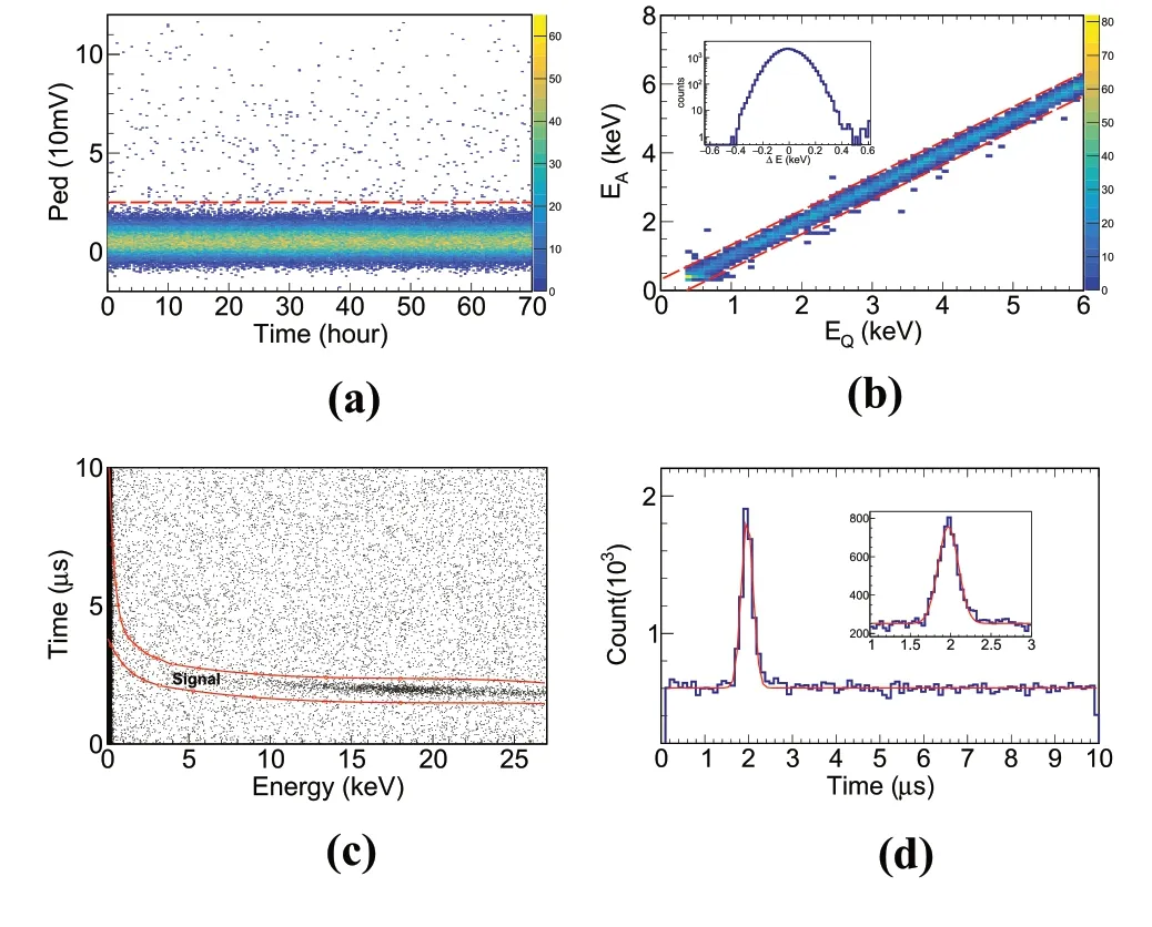
Fig. 6 (Color online) Selection procedures for the recorded data: a Pedestal distribution over time, b Q versus A selection, and c Compton event selection. d Compton signal difference between the two detectors

Fig. 7 (Color online) Influence of each selection in the energy spectrum of HPGe
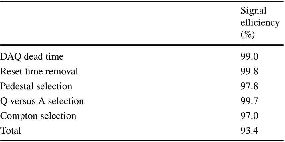
Table 2 Cut efficiency correction
3.QversusAselectionFigure 6b illustrates the relationship between the energy from the pulse integral (EQ)and the energy from the amplitude (EA) of germanium signals. Most events have the sameEQandEA, whereas multi-events in the same time window will have a largerEQthanEA. The energy difference betweenEQandEAis displayed in the inset of Fig. 6b. We selected events within 3σof this distribution, which effectively removed pile up events, and the efficiency was derived as 99.7%using the assumption of a Gaussian distribution.
4.Compton events selectionThe time difference between the NaI and HPGe trigger instant is shown in Fig. 6c,d. The bands correspond to Compton events with the coincidence of germanium and NaI. The dependence on energy was due to the longer time taken for the slowshaping pulse to cross a fixed threshold in the leadingedge discriminator at low energies. The selection effi-ciency was 97% from the survival probability of random trigger events.
We also made two background corrections for the Compton event selection in Fig. 7. One source of background was accidental coincidence. As shown in Fig. 6d, there were almost uniformly distributed events outside the signal range.These events were accidental coincidence events. The other background correction was for coincidence in the surrounding environment. Taking 12◦data as an example, the real Compton events generated by the surrounding environment through the measurement of background data were one-fifth of the total background events.
4.3 Efficiency correction
The selection efficiency of energy-independent cuts, including the DAQ dead time, reset time, pedestal selection, and Compton event selection, derived from the survival of random trigger events, was 93.4%, as shown in Table 2. Energydependent QA cuts derived from the survival of137Cs source events were investigated. The trigger efficiency was derived from the pulse shape of SA2. The maximum amplitude distributions of physics events between 200 and 700 eV are shown in Fig. 8a. The zero-energy point was provided by random trigger events, whereas those for energies below 700 eV were evaluated by interpolation to avoid biased sampling.
The trigger efficiency is defined as the fraction of the amplitude distribution above the discriminator threshold. In Fig. 8b, the black squares represent the trigger efficiency calculated according to the discriminator threshold. The blue line and shaded area represent the hyperbolic tangent function fitting results and the 1σerror band of trigger effi-ciency, respectively. The 50% trigger efficiency corresponds to 198±9 eV.

Fig. 8 (Color online) a Maximum amplitude distributions of physics events between 200 and 700 eV. b Trigger and PSD efficiencies
The pulse-shape discrimination (PSD) efficiency of Q versus A is highly important in the low-energy region. The black circular dots in Fig. 8b represent the PSD efficiency calculated using the experimental signal. The experimental signals in low-energy transfer only contribute a small proportion of the total signals, making the PSD efficiency errors slightly larger. The red line and shaded area represent the hyperbolic tangent function fitting results and the 1σerror band of PSD efficiency, respectively. The 50% PSD efficiency corresponds to 303±19 eV.
4.4 Systematic error
There were two types of systematic errors in the experiment. One was energy-dependent, which changed the profile of the energy spectrum; the other was energy-independent,which did not change the profile of the energy spectrum but scaled it.
The energy-dependent systematic errors originated from the angle-measurement errors and errors caused by the unknown deformation of the collimator. These errors are discussed below.
Systematic error on the calibrated horizontal plane: This error originated from the precision error of the laser-leveling meter. To estimate the horizontal plane error, the laser leveling meter was placed on the horizontal plane and rotated by 90◦several times. At a distance of 5 m, the maximum difference of the emitted horizontal laser lines was 4 mm,from which the plane error was calculated as 0.02◦, consistent with the precision error of 0.3 mm/m given in the laser leveling manual.
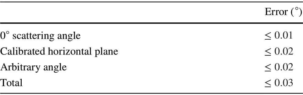
Table 3 Systematic error on the experiment angle
Systematic error on the 0◦scattering angle: The measurements of radioactive sources are shown in Fig. 3 in Sect. 3.The distribution of a radioactive source at 1.499 m and 1.991 m obeyed a Gaussian distribution. The sigma value of the radioactive source was 0.27◦±0.01◦(0.27◦±0.01◦) at 1.991 m (1.499 m). The sigma error of the measured radioactive source in the experiment was 0.15 mm atD= 1.991 m.Mean error of measured radioactive source in experiment is 0.2 mm forD= 1.991 m. We used the measured source distribution, which was Gaussian with (0, 0.27), in the simulations. The error contribution of the radioactive source in the experiment was approximately 0.01◦.
Systematic error on the arbitrary angle: The reason for this error was that the laser emission line had a width of 2 mm. The center position of the NaI detector was determined by the laser line from leveling, whose error was set to a conservative value of 1 mm. Thus, the angle error of NaI located 2 m from the germanium detector was 0.02◦.
The system errors of the angle results are summarized in Table 3. The overall angle errors of the system were constrained and verified at different angles by comparing the experimental and simulation results using the least-squares method. For the experimental angleθ=12◦, the angle confidence intervals derived from simulations compared with the experiment at the 2σconfidence level were 11.99—12.10 for the Livermore model and 11.96—12.03 for the Monash model. These results are consistent with the angle systematic errors below 0.03◦. Therefore, the systematic error on the experimental angle is reliable.
In addition, we studied the effect of the collimator off-set caused by the unknown deformation in the experiment through simulation. The offset of the collimator causes more gamma rays below the 662 keV photoelectric peak to enter the detector, thus affecting the experimental energy spectrum. Limited by the accuracy of the laser level, the collimator offset could be detected when it exceeded 0.3◦.Under the conservative assumption of a collimator offset of 0.3◦, the simulation results showed only a 0.2% difference in the number of events. Thus, this part of the uncertainty was negligible.
Finally, we analyzed the energy-independent systematic errors that affected the experimental energy spectrum.These included multiple triggered events and normalization between the experiment and simulation. The first factor of the energy-independent systematic error was the multiple triggered events. In the experiment, there were many particles incident on the HPGe simultaneously,which led to an undistinguished experimental signal.Therefore, we needed to identify the multiple triggered events in the experiment. Taking the data at 12◦as an example, the number of events triggered by two signals in 8 μs was approximately 27, while the normal event number was 5335. Therefore, the proportion of multiple triggered events was only 0.5%. The second factor of the energyindependent systematic error was the normalization between the experiment and simulation. When comparing the experimental and simulation results, the simulation results should be normalized according to the experimental results. The difference in the total number of events between the Livermore and Monash models, which can affect normalization, was approximately 0.6%, making this part of the uncertainty negligible.
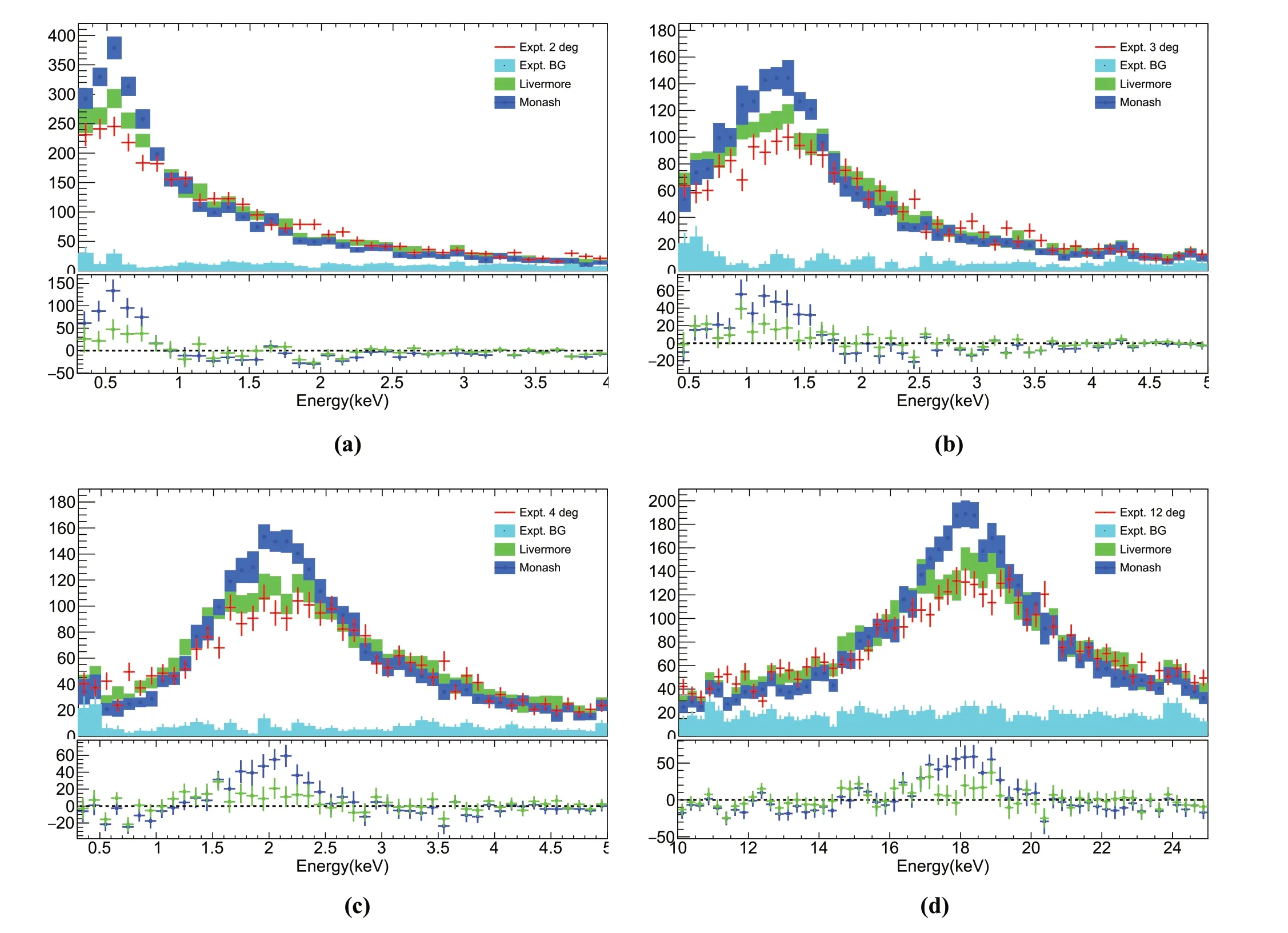
Fig. 9 Experimental results are compared with the simulation results of the Livermore and Monash models
5 Results of the experiment
After processing the experimental raw data using the above procedures, the final experimental data were obtained. This section presents the experimental results for the HPGe detector. To test the consistency between the simulation and experimental results, the experimental conditions shown in Fig. 3 were simulated using Geant4. The experimental results were compared with the simulation results from the DDCS and SDCS of the Compton scattering process.
5.1 Doubly differential cross section
The experimental and simulated results of the DDCS at scattering angleθ=12◦,4◦,3◦,2◦are shown in Fig. 9. The red dots in this figure represent the experimental results.The cyan region represents the background of the experiment. The green and blue lines represent the simulationresults of the Livermore and Monash models, respectively.The least-squares test was used to directly compare the experimental results with the two simulation models.

Table 4 χ2∕ndf under the two models, which were obtained by comparing the experimental energy spectrum with the simulated energy spectrum using the least-squares method

Fig. 10 Comparison of the experimental and theoretical scattering functions. The red line represents our ab initio calculations using MCDF wavefunctions and RIA theory. The blue line indicates the SF results given by Hubbell et al. using HF wavefunctions and Waller—Hartree theory. (Color figure online)
In Table 4, we compare theχ2values of the experimental energy spectrum and simulated energy spectra of the two models. The results included systematic and statistical errors. Atθ=12◦, the Livermore model’sχ2∕ndf=63.2∕60 , and the Monash model’sχ2∕ndf=159.6∕60 . The Livermore model and experimental results were similar (1.79σ), whereas the difference between the Monash model and experimental results was 9.98σ. When the scattering angle was 2◦, the Livermore model’sχ2∕ndf=45.0∕37 , which was significantly better than the Monash model’sχ2∕ndf=137.3∕37 . The difference between the Livermore model and experimental results was 2.83σ, while the difference between the Monash model and experimental results was 10.01σ.
According to the experimental results and least-squares test, the Livermore model is in better agreement with the experimental results.
Because the Livermore model provided results consistent with the experiment, we used the Livermore model as a basis to investigate the effects of SFs on simulations. We employed our SFs calculated using RIA theory and MCDF wavefunctions, as well as the SFs in the Geant4 databases given by Hubbell et al. The least-squares test results indicated that for the DDCS, the two SFs could not be distinguished.
5.2 Singly differential cross section
The SDCS of Compton scattering can be obtained by integrating the experimental spectrum. The experimental SF was acquired by dividing the SDCS obtained from the experimental data into the SDCS of the free electron Compton scattering process obtained in the Livermore model simulation at the same scattering angle.

The experimental and theoretical SFs are shown in Fig. 10.In this figure, the experimental data for scattering angleθ=12◦,4◦,3◦,2◦are plotted.
As indicated in Fig. 10, the experimental SF was closer to our ab initio calculations of SFs at small angles. However,the SF of the Geant4 databases, which was calculated by Hubbell et al., is also within the experimental error. Therefore, the current experimental measurements are insufficient to completely distinguish between the SF of our calculation and Hubbell’s results. In future, we plan to update our experiment to collect more Compton events at smaller angles(θ<2◦). This would be helpful in distinguishing the SF(x<108cm−1).
6 Summary
In this study, we investigated one of the most important background processes in direct DM detection—Compton scattering. Compton scattering has a significant influence on background analysis in direct detection experiments of DM.However, the conventional Geant4 Monte Carlo simulation program uses old atomic databases from nonrelativistic calculations when treating Compton scattering. To provide more precise predictions in Compton scattering background simulations, we used the RIA approach and MCDF wavefunctions to calculate the incoherent SF of germanium atoms. The RIA and MCDF formalisms can effectively treat atomic many-body and relativistic effects. When our ab initio calculations were input into Geant4, the simulation results of Compton scattering in the low-momentum transfer region changed significantly, suggesting that atomic manybody effects significantly influence Compton scattering in low-momentum transfer (sub-keV energy transfer). In addition, we carefully analyzed the simulation results of the Livermore and Monash models in Geant4. These two models use different kinematic methods to simulate the Compton scattering process.
We designed and conducted a high-precision Compton scattering experiment to test the theoretical calculations and simulation results. This experiment employed a coincident detection of HPGe and NaI, and the least-squares test was used to compare the experimental and simulated results.The experimental results showed that the energy spectrum in the Livermore model was in good agreement with the experimental results. It appears that the experimental SF was closer to our ab initio calculations of the SF at small angles. However, the SF of the Geant4 databases calculated by Hubbell et al. is also within the experimental error. In future, we plan to update our experiment to collect more Compton events at smaller angles (θ<2◦). This would be helpful in distinguishing the SF (x<108cm−1).
Our study on Compton scattering may influence X-ray and gamma-ray background analyses in many nuclear and particle physics experiments in future, such as DM detection,the Compton Spectrometer and Imager (COSI) [61], and the Advanced Gamma Tracking Array (AGATA) [62]. A number of simulations could be performed using our improved atomic databases from ab initio calculations. In future studies, we will investigate the effects of Compton scattering backgrounds in direct DM detection experiments, such as CDEX-300, based on simulations of an underground laboratory environment with complicated radioactive sources.
Author contributionsAll authors contributed to the study conception and design. Material preparation, data collection and analysis were performed by Hai-Tao Jia, Shin-Ted Lin, Shu-Kui Liu, Peng Gu and Chang-Jian Tang. The first draft of the manuscript was written by Hai-Tao Jia and Chen-Kai Qiao, and all authors commented on previous versions of the manuscript. All authors read and approved the final manuscript.
杂志排行

Nuclear Science and Techniques的其它文章
- Analysis on the influencing factors of radioactive tritium leakage and diffusion from an indoor high‑pressure storage vessel
- Structural integrity evaluation of irradiated LEU targets for the production of molybdenum‑99 using thermo‑mechanical behavior simulation coupled with pressure of fission gas release calculation
- A method for neutron-induced gamma spectra decomposition analysis based on Geant4 simulation
- Prediction of nuclear charge density distribution with feedback neural network
- Two‑parameter dynamical scaling analysis of single‑phase natural circulation in a simple rectangular loop based on dilation transformation
- Multiple-models predictions for drip line nuclides in projectile fragmentation of 40,48Ca, 58,64Ni, and 78,86Kr at 140 MeV/u