Adaptive composite frequency control of power systems using reinforcement learning

Chaoxu Mu|Ke Wang|Shiqian Ma|Zhiqiang Chong|Zhen Ni

1School of Electrical and Information Engineering,Tianjin University,Tianjin,China

2State Grid Tianjin Electric Power Company Electric Power Research Institute,Tianjin,China

3Department of Electrical Engineering and Computer Science,Florida Atlantic University,Boca Raton,FL,USA

Abstract With the incorporation of renewable energy,load frequency control(LFC)becomes more challenging due to uncertain power generation and changeable load demands.The electric vehicle(EV)has been a popular transportation and can also provide flexible options to play a role in frequency regulation.In this paper,a novel adaptive composite controller is designed to solve the LFC problem for the interconnected power system with electric vehicles and wind turbine.EVs are used as regulation resources to effectively compensate the power mismatch.First,the sliding mode controller is developed to reduce the random influences caused by the wind turbine generation system.Second,an auxiliary controller with reinforcement learning is proposed to produce adaptive control signals,which will be attached to the primary proportion‐integration‐differentiation control signal in a real‐time manner.Finally,by considering random wind power,load disturbances and output constraints,the proposed scheme is verified on a two‐area power system under four different cases.Simulation results demonstrate that the proposed adaptive composite frequency control scheme has a competitive performance with regard to dynamic performance.

1|INTRODUCTION

There usually exist different power generation units and electrical loads in a power system.Frequency deviation is an immediate consequence of the imbalance between the electrical load and the mechanical power supplied to the connected generators.Therefore,the frequency deviation has been a useful index to evaluate the stability of a power system and the quality of electric energy[1].The active power and frequency control are called load frequency control(LFC).When it comes to the power mismatch between generation and demand,LFC plays a fundamental role to restore system frequency,especially for an interconnected multi‐area power system,in which the power mismatch over one control area will affect the frequency of other areas via tie‐lines[2–4].For the purpose of addressing this issue,some LFC designs have been proposed.For example,Yang et al.[5]completed the optimal design of the state feedback matrix and successfully damped the frequency deviation and the tie‐line power fluctuation to zero.By replacing the centralised mechanism with a distributed mode,Ikram et al.[6]proposed a consensus‐based algorithm to estimate power mismatch.In ref.[7],a novel continuous under‐frequency load shedding scheme was presented to eliminate frequency deviation,and this scheme was adaptive to power mismatch based on local frequency measurement.At the same time,in order to increase generation reserves,renewable energy sources(RESs)have been gradually incorporated into the power system.

Various RESs have greatly promoted the development of microgrids,and also facilitated the deep integration of power systems with microgrids.Meanwhile,the increasing penetration of RESs as well as microgrids brings more challenges on frequency stability.The wind turbine generation(WTG)system is a common approach to utilise the endless wind energy,while the wind energy is stochastic and even has large fluctuations in a period of time[8].At the same time,power energy consumption is becoming more and more various.Therefore,for a microgrid,when renewable energy such as wind energy is integrated,it is obvious that there are power mismatch and frequency fluctuation issues.The micro‐turbine is a typical controlled device to compensate for the power mismatch[9],but for a microgrid with renewable energy,it is unrealistic to let the micro‐turbine provide all the active power.It must be supported by some energy storage devices.Typically,EVs can present some positive influences on frequency regulation by acting as energy storage devices when they are spare[10].This paper desires to develop learning‐based LFC controllers to stabilise the frequency of interconnected power systems when the wind turbine and electric vehicles are connected to the power network.Next,some typical LFC methods are reviewed.

The proportion‐integration‐differentiation(PID)controller is a universal regulation strategy for LFC design,and many other control strategies have been applied to deal with the frequency regulation problem,such as robust control,optimal control,sliding mode control(SMC),and so on[11–15].Among them,Sathya et al.[13]proposed an improved PID frequency control method using the Bat inspired algorithm.Based on the SMC structure,Mi et al.[14]designed an LFC controller for the multi‐area power system with matching and mismatching uncertainties.In ref.[15],a distributed optimal control method was proposed to restore the nominal frequency as well as the tie‐line power flows between control areas after the power mismatch.On the other hand,some adaptive and intelligent control algorithms have been reported in power systems[16–19].Among them,Dash et al.[17]proposed an adaptive neural network(NN)control method to adjust frequency fluctuations.In ref.[18],an adaptive fuzzy logic controller was designed to stabilise the frequency.Similarly,Yousef et al.[19]also proposed an adaptive fuzzy frequency controller.These research studies preliminarily show the potential of learning‐based methodologies in the LFC design.Unlike these studies,this paper is devoted to designing a learning‐based controller in the optimal sense,and hence focuses on a learning technique called adaptive dynamic programing(ADP).

Adaptive dynamic programing employs the knowledge of reinforcement learning and dynamic programming to complete an optimal control design by minimising a designed cost function.This learning technique usually adopts neural networks to approximate non‐linear functions and has been applied in various industrial fields[20–23].In recent years,some ADP‐based control methods have been developed to regulate the frequency of power systems.For example,in ref.[24],the frequency stability of an isolated smart grid was studied based on goal‐representation ADP approach.Lu et al.[25]obtained better control performance in stabilising a large power system.Sui et al.[26]effectively suppressed frequency oscillations for a power system when considering energy storage devices.In ref.[27],a novel fuzzy ADP‐based controller was also developed when considering the transmission delay,so as to increase the transient stability.In addition,we found some studies on the LFC problem of microgrids to be inspiring for our work.For the microgrid containing photovoltaic,Sekhar et al.[28]proposed a tracking mechanism based on adaptive predictive correction to adjust the frequency.In ref.[29],by using centralised and distributed coordinated control methods,the primary frequency regulation of the microgrid was solved by simultaneously introducing wind turbines and EVs.

The above‐mentioned articles have successfully addressed the frequency stability problem of the power system to a certain extent;however,there still exist some challenges to be tackled:(1)dynamic response ability of the system frequency needs to be enhanced,and the controller needs to be further optimised;(2)more generic and effective LFC designs are required for multi‐area power systems by considering the integration of wind energy and electric vehicles;(3)Most intelligent controllers are purely designed based on learning techniques and have no consideration for the stability margin;besides,the frequency regulation process lacks optimality considerations.With the aid of ADP,proposing an efficient LFC method to solve these problems is the main motivation behind this work.

This paper considers an operation scenario in which wind energy and EVs are included into the multi‐area power system,and thus a composite frequency controller is proposed which consists of a PID primary signal and ADP‐based auxiliary signal.The main contributions include the following:(1)A novel hybrid LFC model is constructed for the multi‐area interconnected power system,in which the wind turbine and electric vehicles are integrated on the basis of traditional governor‐turbine units.(2)A sliding mode pitch angle controller is designed for the WTG system,which is integrated into the inner loop of the power system to provide positive active power;besides,electric vehicles are introduced in the form of EV aggregators to effectively support the frequency regulation.(3)Based on PID and ADP,an adaptive composite frequency control scheme is proposed for the wind‐integrated multi‐area power system,in which the auxiliary adaptive control is implemented by the action‐critic NN structure and reinforcement learning mechanism.

The rest of paper is arranged as follows:Section 2 describes the multi‐area power system and states the LFC problem and then designs the pitch angle controller for the WTG system.Section 3 introduces the detailed design process of the PID primary controller and learning‐based auxiliary controller.Section 4 performs some simulation cases on a two‐area power system,and all the simulation results are comparatively analysed.Finally,Section 5 concludes this work and provides some future insights.

2|SYSTEM DESCRIPTION AND PROBLEM FORMULATION

2.1|The load frequency control problem of hybrid multi‐area power system

The LFC model of a classic multi‐area power system is mainly composed of governors,turbines,electric loads and tie‐lines.Although power systems indeed have a non‐linear and time‐varying nature,for the purpose of frequency analysis in the presence of load disturbances,the linearisation model is usually adopted[9].This is accounted for the fact that the system presents an obvious linear property around a rated operating condition[1].After considering wind turbine and EVs,a block diagram of the LFC model used for a hybrid multi‐area power system is shown in Figure 1,in which each component is described by the transfer function.It can be seen that each control area contains a governor‐turbine unit,EV aggregators,wind turbine,power system(namely electricity consuming system),frequency controller,pitch angle controller,electric loads and tie‐lines.Each two areas transmit power through the tie‐lines.Moreover,in each area,the turbine unit and WTG system provide active power,and EVs also contribute to the active power.At this time,this power system can also be seen as a microgrid.Next,the main signals and variables in each area are introduced.

For thei‐th area,Δfiis the frequency deviation,Tit,TigandTipare the time constants of the turbine,the governor and the power system,respectively.Tijrepresents the interconnection gain or synchronising power coefficient between areasiandj.ΔPitandΔXigdenote the turbine power and the governor position valve,respectively.ΔPie1,…,ΔPienare the change of EVs power,andTie1,…,Tienare the time constants of EV aggregators,where each EV aggregator supervises an EV group.Ri,KifandKipare the speed regulation coefficient,gains of frequency deviation and power system,respectively.ΔPid,ΔPiwgandΔPtie,iare the disturbances from load change,WTG system and tie‐line power deviation,respectively.The power system achieves electric energy balance through automatic generation control(AGC)to meet the frequency stability under load fluctuations.Since only one generation unit is involved in each area,the AGC does not need to consider the distribution coefficient.The balance between interconnected control areas is achieved by detecting the frequency and tie‐line power deviations to generate the area control error(ACE)signal,given by

It is evident that the ACE signal is a linear combination ofΔfiandΔPtie,iand is in turn utilised in the controller design.Therefore,the purpose of the controller is to adjust both the frequency deviation and the ACE to zero.

Remark1 Note that in a microgrid,the electric loads not only refer to commercial and industrial loads,such as supermarkets and factories,but also have some new types of loads,such as smart homes.They can be regarded as load disturbances,and therefore in the simulation analysis,different step disturbances are usually added to observe the frequency deviation[30].

Remark2 Electric vehicles are integrated into the power system and can be seen as energy storage devices,which are regulated by EV aggregators[31].Aggregator is the concept of EV clusters.Although a single EV is uncertain,the EV cluster composed of multiple electric cars will exhibit certain statistical regularities,and its uncertainty will be greatly reduced.It is also worth emphasising again that both electric vehicles and the wind turbine provide active power[32],and hence the influences of wind energy and electric vehicles are considered as positive power disturbances.

2.2|Effect of electric vehicles on the frequency regulation

In this section,the impact of EVs on the frequency response is discussed.EVs act as distributed storage devices and respond to frequency changes by transmitting energy to the power system.

FIGURE 1 Structure sketch of the i‐th area in a multi‐area power system

FIGURE 2 Frequency deviation and power mismatch

In order to illustrate the effect of EVs,the relationship between frequency deviationΔfand total power mismatchΔPis shown in Figure 2.[ΔfL,ΔfU]and[ΔPL,ΔPU]are acceptable ranges of frequency deviation and total power mismatch,respectively.EVs are controlled to enhance their charging power whenΔfexceeds the upper bound valueΔfU,such asCase Ain Figure 2;conversely,EVs are controlled to enhance their discharging power whenΔfexceeds the lower bound valueΔfL,such asCase Bin Figure 2.In this way,EVs can effectively reduce the total power mismatch of power system[33],and hence support the generation unit to compensate for the power imbalance.In addition,compared to common energy storage systems,EV stations are easy to manage and relatively low in operating costs.Therefore,it is of significance to investigate the co‐design of electric vehicles and WTG system on the frequency response.

2.3|Sliding mode pitch angle controller

In this section,we analyse the power output of the WTG system and design the corresponding controller.Due to the randomness of wind energy,the output power of the WTG system is usually fluctuating and even unstable[34].Therefore,it is necessary to stabilise the output power of the WTG system before it is connected to the grid.Pitch angle control is the most popular approach against wind power fluctuation[35].In this work,a sliding mode pitch angle controller is proposed to reduce power fluctuations.This controller will behave as the block‘pitch angle controller’shown in Figure 1.

The whole WTG system mainly includes three parts:wind turbine,hydraulic servo system and pitch angle control system.First,the output of wind turbine can be calculated by

wherePwis the output power andCp(λ,β)is the power coefficient,in whichλandβare the tip speed ratio and the pitch angle,respectively.Besides,v,ρandℏare the wind speed,the air density and the blade radius,respectively.

The power coefficientCp(λ,β)is expressed by

withci(β)=ci0+ci1β+ci2β2+ci3β3+ci4β4;i=1,2,3,whereci0,…,ci4are the parameters determined by the characteristics of the wind turbine.The tip speed ratio is

whereωis the angular velocity and can be calculated by

In Equation(5),Mis the inertia moment of the wind turbine.In this design,WTG is used as a squirrel‐cage induction generator[36],and the output powerPwgcan be calculated by

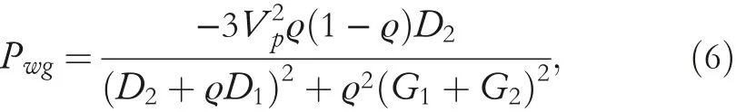
whereVpis the phase voltage;G1andG2are the reactances of the stator and rotor,respectively;D1andD2are the resistances of the stator and rotor,respectively.Also note thatϱ=(ω0−ω)/ω0is the slip of the induction generator,whereω0is the synchronous angular velocity.In this paper,the pitch angle of wind turbine is from 10°to 90°and will be regulated by the sliding mode controller.

Next,one considers such a relationτw=Pw/ω,whereτwis the output torque of the wind turbine and can be given by

where Equation(2)has been used.In order to design a controller,τwneeds to be linearised around the rated operating point,which is denoted byτwop=f(wop,βop,vop),whereωop,βopandvopare steady‐state or rated values ofω,βandv,respectively.With the help of Taylor expansion,(7)can be linearised as follows:

with

whereΔω=ω−ωop,Δβ=β−βopandΔv=v−vop.Note that during this process,the higher‐order items have been ignored.

The dynamic model of WTG system can be expressed as

whereτwgis the generator torque.Also note that at a specific operating point,the turbine and generator torques are assumed to be the same.Thus,by considering Equations(8)and(9),the model of the WTG system can be formulated as

At this point,the linear model of the WTG system is obtained and then we can proceed to design the sliding mode pitch angle controller.First,the sliding mode variableξis defined as

with a constant gainς.Since the pitch angle controller works only when the output powerPwgis greater than the rated powerPrg,soΔω>0 can be obtained.

By adopting the reaching law=−ηξ−εsat(ξ)[37],the sliding mode pitch angle controller is designed as

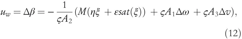
whereηandεare positive constants,sat(ξ)is the saturation function to reduce the chattering.Define the Lyapunov function asthen we can obtain

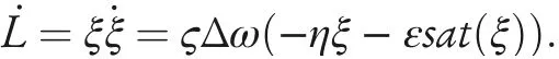
SinceΔω>0,we can know that≤0.Based on the Lyapunov stability theory,it is concluded that the designed sliding mode pitch angle controller can let the WTG system be asymptotically stable.

Until now,the integration of wind energy is solved and the corresponding controller has been designed.In the next section,we will design a learning‐based composite LFC controller.

3|ADAPTIVE‐CRITIC‐BASED COMPOSITE DESIGN FOR FREQUENCY REGULATION

The proposed control strategy utilises the PID signal as the primary control signal while introducing an adaptive critic signal to adjust the dynamic response.This adaptive critic control scheme is implemented by the heuristic action‐critic NN structure.The adaptive critic mechanism is elaborated as follows:

The critic NN estimates the cost function,which is composed of the control cost and the environment reward[38].The action NN updates the control signal under the estimated cost function,so that the control signal can be adaptive to the system.First,the cost function is defined by

whereU(x(t),u(t),t)is the utility function,in whichx(t),u(t)andγare the state vector,control signal and discount factor,respectively.

Second,using the Bellman optimality principle yields the optimal cost functionJ*(t)given by

whereJ*(t)andJ*(t+1)are minimum cost functions for the corresponding time.From equation(14),one can observe that it is not easy to get the optimal control signalu*(t)since the future costJ*(t+1)cannot be known prior.In our design,two NNs are applied to solve this equation(14)such that the optimal control signalu*(t)can be approximately obtained forward in time.

3.1|Critic neural network

The critic network is implemented by a single‐hidden‐layer NN,shown in Figure 3,wherekcandmcare the neuron numbers of the input and hidden layers,respectively.The sigmoid function is used as the activation function.For an independent variablez,it is

Specific to the multi‐area power system,the cost functionJi(t)is defined for thei‐th area:

whereuia(t)is the adaptive auxiliary control,which can be approximately estimated by the action NN.xia(t)is the state vector generated by frequency deviations.Therefore,the input vectorxic(t)∈Rkcof critic NN is denoted by

By using the critic NN,Ji(t)can be estimated by

FIGURE 3 Critic neural network(NN)structure

wherewc1κι(t)is the input‐hidden weight;wc2ι(t)is the hidden‐output weight;pcι(t)andqcι(t)are intermediate variables;and(t)is the estimation of cost function.At this time,the approximation error or learning error is defined as follows:

which can be driven to zero by minimising such a squared error

Based on this squared error,one only needs to design appropriate weight updating rules to make the actual cost^Ji(t)approximate to the optimal cost function.For this purpose,the back‐propagation‐based gradient‐descent method is adopted,and thus the updating rule of the hidden‐output weight vector is given by

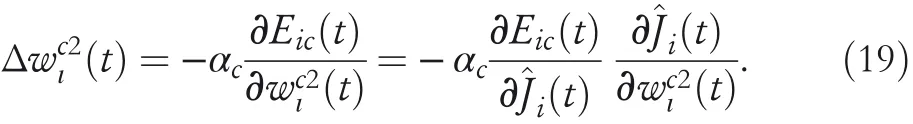
Similarly,using the chain rule,the input‐hidden weight vector is updated by

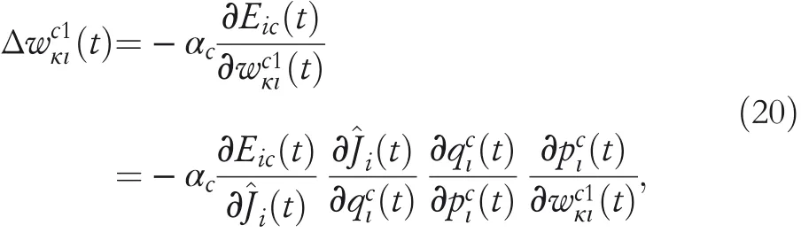
whereαcis the corresponding learning rate,κandιsatisfyκ=1,…,kcandι=1,…,mc,respectively.

3.2|Action neural network

The implementation of an action NN is similar to that of a critic NN.A three‐layer NN is taken as the action NN withkainput‐layer neurons andmahidden‐layer neurons.The participant frequency regulation variables constitute the input vectorxia(t),which is

With this input vector,the action NN generates an auxiliary control signaluia(t),given by

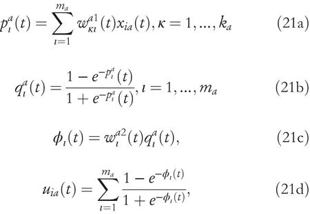
wherepaι(t)andqaι(t)are the input and output values ofι‐th hidden‐layer neuron.wa1(t)is the input‐hidden weight vector andwa2(t)is the hidden‐output weight vector.For the action NN,its learning error is defined by

whereUd(t)is the desired cost and is usually set as 0.Similarly,this error is driven to zero by minimisingEia(t)=1/2e2ia(t).Using the gradient‐descent method,the weight vectorcan be adjusted according to

and(t)is updated by

whereαais the corresponding learning rate.It is worth emphasising that although the optimal solution is obtained in an approximate manner,this heuristic ADP algorithm can ensure that the stability result is uniformly ultimately bounded(UUB),along with the weight convergence.This property has been proved in ref.[39].

3.3|Adaptive‐critic‐based composite frequency controller

In this section,we present how to implement the composite control scheme and provide some discussions on the proposed method.

FIGURE 4 Schematic block diagram of the i‐th area power system with a composite control scheme.(The data processing module is to collect the frequency deviation and its time delays such that the system vector can be obtained.In this design,the state vector xia(t)is composed ofΔfi(t)andΔfi(t−1),that is,xia(t)=[Δfi(t),Δfi(t−1)]T.)

For each area,the primary PID controller and auxiliary controller together constitute the composite frequency controller,namely the block‘frequency controller’shown in Figure 1.Furthermore,a simplified block diagram with this novel composite control strategy is presented in Figure 4.It can be seen that the overall system has two controllers:the sliding mode pitch angle controller reduces the wind power fluctuations,and the composite frequency controller regulates the outputs of turbine and EV aggregators to reduce the power mismatch.In this case,the composite control signalui(t)is obtained by adding the primary control signalui0(t)and the auxiliary control signaluia(t),which is constrained into a certain range.

In the auxiliary controller,action and critic NNs are applied to generate the auxiliary adaptive control signal and approximate the associated cost function.Specifically,in this paper,the input vector of the auxiliary controller is

whereΔfi(t)andΔfi(t−1)are the frequency deviation at timetand its one‐step time delay,respectively.

For each area,the utility function is defined by

whereri(t)is the reward signal and is calculated by

It is evident thatri(t)is composed of different frequency deviations and hence can be used to evaluate the performance of auxiliary control signaluia(t).When load disturbances occur,the system frequency will deviate from its specified value and then the reward signalri(t)will also change.For example,ri(t)will become larger whenΔfi(t)becomes larger.This design takes into account the demands for system stability and dynamic response.As a result,the adaptive ability of the frequency controller will be greatly improved by adding the learning‐based control signal.

Remark3 PID controller plays a fundamental role in stabilising the frequency and eliminating the steady error,while the auxiliary ADP controller is responsible to speed up the frequency regulation process by improving the dynamic response.

The working procedure for regulating the system frequency of thei‐th area is summarised in Algorithm 1.During the learning process,two iteration criteria are adopted,that is,the maximum number of iteration steps(Mc,Ma)and the minimum allowable error(εc,εa).

Algorithm 1 Learning-based composite control procedure for frequency regulation of a multi-area power system 1:Let the running time be T=70 s and the criteria be Mc=80,Ma=50,εc=εa=1e−5.Initialise two NNs and obtain the initial control signal uia(t).2:With xia(t),uia(t)and the reward signal ri(t)given in Equation(26),the critic NN approximates the cost function^Ji(t).3:According to the^Ji(t)and^Ji(t−1),calculate two network learning errors by using Equations(18)and(22).4:By using Equation(19),(20),(23)and(24),update the network weights until the criteria are satisfied.5:Calculate the new control signal using the obtained weights and go into the next sampling period.6:Obtain the composite control signal by adding uia(t)and ui0(t),and then use it to adjust the frequency.7:Repeat the above steps at each sampling time until the simulation time arrives.

Until here,the LFC model and control scheme of the overall system have been completed.Before starting the simulation,some characteristics of the proposed adaptive composite frequency control are summarised in the following remarks.

Remark4 The design parameters of the composite frequency controller are mainly reflected in two aspects:PID parameters and learning parameters related to the auxiliary controller.For PID parameters,one can select corresponding gains using the classical tuning method.As for the auxiliary controller,it mainly contains network parameters(kc,ka,mc,ma),learning rates(αc,αa),weight matrix(Q)and the discount factor(γ).It is recommended to select four network parameters within[2,10],because the current system is not particularly complicated.Two learning rates can be given relatively small values according to the specific operating condition.The matrix Q is generally selected to be a positive definite matrix.The discount factor can be randomly selected within(0,1),and we recommend it to be greater than 0.8.

The parameter selection of the sliding mode controller is relatively free.It mainly contains three positive parameters(ς,η,ε),and one can select relatively small values for them.

Remark5 The differences and advantages of the presented control algorithm are mainly reflected in two aspects:1)Compared with ref.[14,15],our design considers the learning property,which enables the adaptability and optimisation abilities to the controller;2)Compared with learning designs in ref.[4,24,40],our control algorithm is implemented on the basis of PID,which guarantees the basic frequency response performance and avoids negative influences caused by poor learning results.

Remark6 Note that the current control design does not consider dead‐time and time‐delay,but considers some output constraints,so as to specifically observe the performance of the learning‐based controller.However,the dead‐time potentially exists in the controller,and sometimes it will seriously affect the system stability.When it comes to the dead‐time,an extra control compensation mechanism may be effective in suppressing undesirable effects.

Remark7 Also note that although some output constraints are considered,the whole LFC model is still a linear control system,and hence the primary PID controller can effectively ensure stability.In addition,the auxiliary ADP‐based control method can obtain the result of UUB stability.Therefore,the overall system stability can be ensured under the proposed composite control scheme.

4|SIMULATION AND ANALYSIS

A two‐area power system is used to illustrate the performance of the proposed frequency controller in this section.Note that each area includes two EV aggregators and a pitch angle controller.The capacity of each control area is the same and the output power unit is denoted byp.u.MW;besides,the nominal system frequency is 50 Hz and the frequency deviation unit is denoted byp.u.Hz.It is assumed that the power network initially operates at a nominal point,and the frequency response is observed by adding load disturbances.Each area is equipped with a composite frequency controller to regulate the governor‐turbine unit and EVs,and the output signal of the auxiliary controller is limited to the interval[−0.01,0.01].The simulation parameters for the two‐area power system are listed in Table 1.

All simulations are conducted on the Simulink platform of MATLAB R2020b.The computer processor is Intel(R)Core i5‐10,400F CPU@2.90 GHz,and a 70 s frequency response simulation takes approximately 6.5 s of CPU time.

In order to intuitively evaluate the dynamic performance of frequency regulation,four evaluation indexes are used:

(1)Maximum overshoot(MOV)of frequency deviation:max(Δfi).

(2)Minimum undershoot(MUN)of frequency deviation:min(Δfi).

(3)Standard deviation(STD)of frequency deviation:

whereNis the total number of data points,andΔfiis the mean value ofi‐th area frequency deviation.

(4)Integral absolute error(IAE)of frequency deviation:

These indexes are widely adopted to judge the dynamic performance of the LFC controller[30],and for these four indexes,a smaller value means a better performance.

In order to comprehensively examine the proposed composite control method,four simulation cases are considered in this section.Specifically,Section 4.1 verifies the effectiveness of the sliding mode pitch angle controller;Section 4.2 verifies the effectiveness of the composite frequency controller;Section 4.3 tests the frequency regulation effect of electric vehicles under random load disturbances;and finally,Section 4.4 investigates the adaptive performance under parameter uncertainties.

4.1|Control performance of wind turbines

In this case,the performance of the sliding mode pitch angle controller is analysed to observe whether it can maintain the wind turbine around its rated power.We selectA1=−5794,A2=10,607,A3=−2263 and coefficientsCpaccording to ref.[36].Other related parameters of the WTG system areprovided in Table 2.In the sliding mode controller,ς=0.01,η=0.01 andε=0.1;besides,the PI pitch angle controller is used for comparison,where the proportional gain isKP=0.4 and the integral gain isKI=0.6.

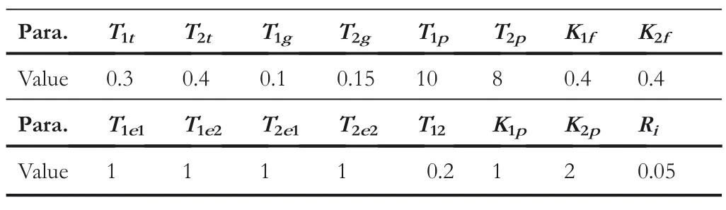
TABLE 1 The parameters of two‐area power system

In the simulation,the random wind speed is generated by the Kaimal wind power spectrum[41],which is shown in Figure 5.The wind speed is considered to be higher than its rated value,but lower than the cut‐out wind speed,which is set to 25 m/s.

From Figure 5,it can be seen that the wind speed is random and rapidly fluctuating.Despite this,power stability of the WTG system can be effectively maintained using the sliding mode controller,which can be confirmed from the wind power error signalΔPwgas shown in Figure 6.Moreover,the tendency of wind power is consistent with that of wind speed,which is higher(or lower)than the rated power when the wind speed is higher(or lower)than the rated wind speed.Compared with the PI controller,the sliding mode controller has smaller fluctuations and is more effective in stabilising the output power of the WTG system.

4.2|Dynamic response for disturbances and output constraints

In this case,synthetic disturbances and output constraints are considered at the same time.The PID controller is applied to stabilise the frequency at the specified value while the adaptive auxiliary is used to ameliorate dynamic performance.The parameters of the auxiliary controller are set asαc=αa=0.05,Q=diag{1,0.5},kc=3,ka=2,mc=ma=6 andγ=0.95.For comparison,the PID controller is also individually applied to control the same hybrid two‐area power system.The gain parameters of PID controllers are selected asKP1=15,KP2=5,KI1=26,KI2=20,KD1=1 andKD2=4.Meanwhile,for area 2,the turbine output constraint is[−0.12,0.12]p.u.,and the output constraints of two EV aggregators are[−0.04,0.01]p.u.and[−0.035,0.01]p.u.,respectively.

Moreover,it should be emphasised that in all available standards,the acceptable frequency deviation for normal operation is relatively small(about 1%,refers to[1]),and hence it desires to control the frequency deviation within±0.5 Hz,namely±0.01p.u.Hz.

As hinted before,it is assumed that the power network initially operates at a nominal point,and two load disturbances−0.12p.u.and+0.16p.u.will be sequentially introduced at 10 sand at 40 s,respectively.After adding the wind power error shown in Figure 6,the synthetic disturbances can be obtained as presented in Figure 7.Under the synthetic disturbances,the frequency responses produced by the PID controller and composite controller are presented in Figure 8,and two adaptive auxiliary control signals are given in Figure 9.In order to reveal the weight regulation,Figure 10 is provided to present the weight updating process ofwc1211,…,wc1216for the auxiliary controller used in area 2.The adjustment of other weight vectors is similar and is thus omitted.

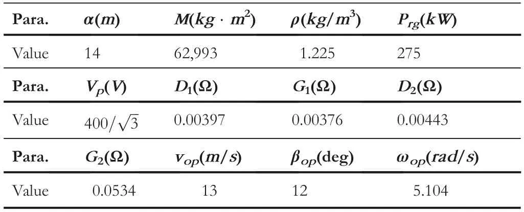
TABLE 2 The parameters of the wind turbine generation(WTG)system

FIGURE 5 Wind speed v

FIGURE 6 Output power error of wind turbine generation(WTG)system Pwg

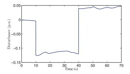
FIGURE 7 Synthetic disturbances from load change and wind turbine generation(WTG)system

FIGURE 8 Frequency response of a two‐area power system with output constraints:(a)Comparative frequency responses of area 1;(b)Comparative frequency responses of area 2

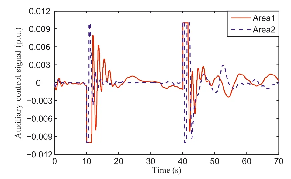
FIGURE 9 Adaptive auxiliary control signals of a two‐area power system with output constraints

It can be observed from Figure 8 that compared with the PID controller,the composite controller has the ability to stabilise the frequency deviation faster with smaller overshoots and fewer oscillations for both areas.In addition,due to the impact of output constraints for area 2,the frequency response of area 1 is slightly better than that of area 2.As stated before,to avoid oversized outputs,two supplementary adaptive control signals are limited to suitable ranges,shown in Figure 9.It can also be observed from Figure 10 that the learning process corresponds to the changes of synthetic disturbances.

Next,we transfer to analyse the output power of this two‐area power system.In our settings,area 1 does not consider output constraints.The output power of the turbine in area 1 is displayed in Figure 11a.Due to the fact that the first EV aggregator and second EV aggregator are the same,only the output power of the first EV aggregator is given in Figure 11b.For area 2,the output power of the turbine and two EV aggregators are presented in Figure 12a–c.It can be evidently seen from each close‐up,the output power of the turbine has been constrained within[−0.12,0.12],and the EVs are also strictly limited to[−0.04,0.01]and[−0.035,0.01].

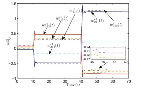
FIGURE 1 0 Weight updates of critic network for area 2

FIGURE 1 1 Output power of area 1:(a)Output power of the turbine;(b)Output power of the first EV aggregator

Finally,in order to compare these two methods more intuitively,we analyse the dynamic performance from the perspective of data.For this frequency regulation process,four evaluation indexes of two methods are listed in Table 3.It can be seen that in two areas,regardless of overshoot,standard deviation or accumulated error,the proposed composite controller can obtain relatively small values.This indicates that its dynamic performance is better because the data volatility is relatively small.Furthermore,it can be found that the composite controller can stabilise the frequency around±0.5 Hz,while for the PID controller,the frequency deviation in area 2 will exceed−0.5 Hz(−11.14p.u.Hz×10−3×50=−0.56 Hz).Based on the aforementioned results and discussions,it can be concluded that the composite controller is superior to the PID controller.

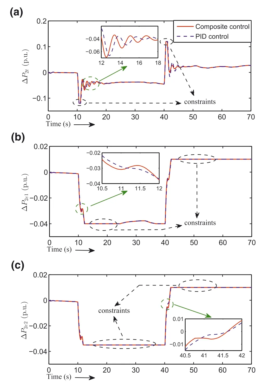
FIGURE 1 2 Output power of area 2:(a)Output power of the turbine;(b)Output power of the first EV aggregator;(c)Output power of the second EV aggregator

TABLE 3 Comparison of frequency response results from Figure 8(10−3p.u.)

4.3|The frequency regulation effect of EV aggregators under random load disturbances

In general,the load of the power system regularly changes as the actual demand;however,the white noise may remain present in the load disturbances due to the continuous switching operations.Therefore,it is necessary to investigate the proposed scheme in the presence of random disturbances[30].On the other hand,in order to show the regulation effect of EVs,we also performed comparative results with EVs and without EVs under composite control scheme.The frequency responses are provided in Figure 13.

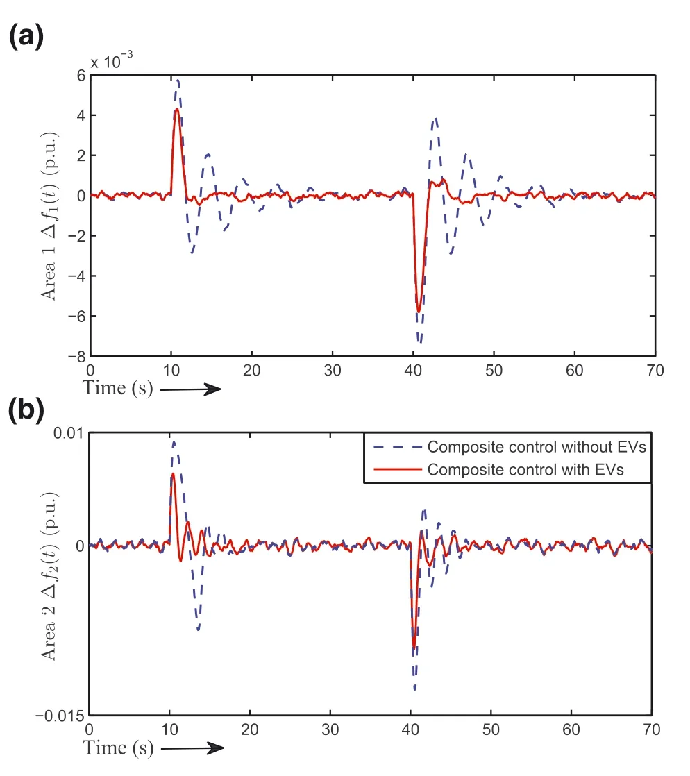
FIGURE 1 3 Frequency response of two‐area power system under random load disturbances:(a)Comparative frequency responses of area 1;(b)Comparative frequency responses of area 2

TABLE 4 Comparison of frequency response results from Figure 13(10−3p.u.)

In this case,the system frequency is not only subject to the synthetic disturbances shown in Figure 7,but is also affected by the white noise of a small magnitude.It can be observed that for the composite controller with EV aggregators,the frequency regulation is more superior due to fewer fluctuations and smaller overshoots.It can also be observed that the whole response process is accompanied by minor oscillations,while it is overall stable.Moreover,associated evaluation indexes are listed in Table 4.It is evident that due to small persistent disturbances,the IAE will become larger at this time;but for the controller with EVs,all frequency deviations still lie in the allowable range(the MUN is−9.156p.u.Hz×10−3×50=−0.46 Hz).However,if electric vehicles are not introduced,the frequency deviation in area 2 will exceed−0.5 Hz(−12.73p.u.Hz×10−3×50=−0.64 Hz),and hence it is obvious that EV aggregators can effectively compensate for the power mismatch.It is thus concluded that the proposed composite control scheme can stabilise the frequency even for random load disturbances,and will perform better when EVs are participating.

4.4|Adaptive ability analysis for composite control

Generally,there are parameter uncertainties in the power systems.In order to verify that the designed composite controller has good robustness and adaptability when facing system parameter changes,it is considered that the time constants of governors and EV aggregators have been deviated(these deviations are set within±20%).The comparison is illustrated by two scenes,and their specific parameter settings are given in Table 5.

The scene in Section 4.2 is termed as the Scene‐N,whose frequency responses have been given by Figure 8.On this basis,we keep PID parameters unchanged and then performthe dynamic response of Scene‐A,thereby obtaining the corresponding results in Figure 14.In Scene‐A,the PID parameters are the same as Scene‐N and are fixed while only the adaptive control signal can make responses to the parameter changes.The corresponding evaluation indexes for this case are listed in Table 6.

TABLE 5 The parameters of two scenes

FIGURE 1 4 Frequency response of Scene‐A:(a)Comparative results of area 1;(b)Comparative results of area 2

TABLE 6 Comparison of frequency response results from Figure 14(10−3p.u.)

The PID parameter tuning is completed in Scene‐N,so this strategy performs relatively poor in Scene‐A.Observing Figure 14,the fluctuations of PID control are significantly more dramatic while composite control can still obtain favourable dynamic responses.Because the composite control scheme contains an auxiliary adaptive controller that can handle parameter changes within small ranges,even if the primary controller is not re‐tuned,it can still adjust the response process.In addition,from Table 6,one can tell that the frequency deviations of two control methods are all located in the range±0.5 Hz,while composite control still performs better.Hence,another significance of the proposed composite control lies in better robustness or adaptability for small parameter changes.

In summary,the proposed composite control method not only controls governor‐turbine units and EV aggregators to eliminate the frequency deviation,but also use the auxiliary control signal to improve dynamic performance through reinforcement learning.

5|CONCLUSION

In this paper,a novel composite frequency control scheme is proposed for the multi‐area power system,where wind power and EVs are simultaneously considered.In the constructed hybrid LFC model,a sliding mode pitch angle controller is used to maintain the output power of the WTG system,and electric vehicles participate in the frequency regulation in the form of EV aggregators.In order to improve the frequency response,an auxiliary controller is designed based on the knowledge of ADP,which gives adaptive control signals by implementing reinforcement learning scheme.After combining it with a PID controller,the composite controller can be obtained.In the simulation,four different cases are considered to illustrate the effectiveness of the proposed method on a two‐area power system.Comparative simulation results demonstrate that the proposed composite control scheme not only stabilises the frequency within the acceptable range but also has better performance with regard to frequency regulation,random load disturbances and parameter uncertainties.

Despite this,the current design still has some disadvantages:(1)it has no ability to deal with complicated non‐linear conditions,such as dead‐time and generation rate constraints etc.;(2)lack of consideration of the communication problem between different areas;and(3)the current design of reinforcement learning fails to consider the cooperative behaviour.In future work,we may improve reinforcement learning algorithms using different NN structures(such as those reported in ref.[42,43])to address complicated non‐linear conditions while considering event‐triggered control to cope with limited communication resources.

ACKNOWLEDGEMENTS

The work is funded by the science and technology project of SGCC(State Grid Corporation of China)(5700‐202,212,197A‐1‐1‐ZN).

CONFLICT OF INTEREST

The author declares no conflict of interest.

DATA AVAILABILITY STATEMENT

The data that support the findings of this study are available from the corresponding author upon reasonable request.

ORCID

Chaoxu Muhttps://orcid.org/0000-0003-1055-9513

Ke Wanghttps://orcid.org/0000-0002-8306-1663

Zhen Nihttps://orcid.org/0000-0003-3166-4726