Modelling of a shape memory alloy actuator for feedforward hysteresis compensator considering load fluctuation
2022-12-31SeijiSaitoShoutaOkaRibunOnodera
Seiji Saito |Shouta Oka|Ribun Onodera
Abstract This paper presents a hysteresis mathematical model of a shape memory alloy(SMA)actuator for feedforward hysteresis compensator.The hysteresis model represents the relation between temperature,stress,and electric resistance.Firstly,based on the laws of thermodynamics,the hysteresis model of the SMA actuator is built.Secondly,the inverse of the hysteresis model is obtained to produce a compensator for non‐linear characteristics such as hysteresis and saturation.Thirdly,the parameters of the hysteresis model are obtained from each experiment under constant load and constant temperature,and the model validity is confirmed by comparing experimentally obtained results.Finally,the inverse model is applied to a part of feedforward hysteresis compensator.In order to verify the effectiveness of the proposed model as hysteresis compensator,an electrical resistance control using feedback–feedforward control was conducted by numerical simulation.The simulation results indicate advantages of the proposed mathematical model in hysteresis compensation of SMA actuator,and demonstrate that the model is capable of handling load fluctuation.
1|INTRODUCTION
In recent years,energy conservation and small size have come to be valued as characteristics for sensors and actuators used in industrial fields.Smart materials have attracted a particularly great deal of attention for making sensors and actuators even more energy efficient and compact.The mechanical and electrical properties of smart materials are altered by external stimuli such as force,temperature,light,and magnetic fields.Smart materials can work as sensors and actuators by taking advantage of the change in the properties;they are anticipated for use as a substitute for existing sensors and actuators to provide energy conservation and small size.
Smart materials include magnetostrictive materials,piezoelectric materials,and electroviscous fluids.Shape memory alloy(SMA)is also included in smart materials,which is highly anticipated for use as an actuator material.Actually,SMA can generate the highest stress and strain of any actuator material.Moreover,SMA has the property of transforming into a specific shape.Strain in SMA results from two mechanisms:the shape memory effect(SME),whereby heating of a deformed SMA causes it to return to its pre‐deformed shape;and the superelastic effect(SE),whereby deformation of a heated SMA generates strain that causes shape‐reversion when unloaded[1].
Length of wire‐type SMA(SMA wire)actually decreases when heated by Joule heating with application of an electric current.Shape memory alloy wire has many applications,and has been specifically used in artificial muscles[2,3],robots[4–6],and medical equipment[7,8].These are some examples of how such strain is used in industrial equipment.For strain control using SMA wire,measuring the strain directly in a real system is not easy,and the mechanism becomes very complicated when extra strain sensors are used.Therefore,many attempts have been made to model the relation between strain and electrical resistance and to control strain indirectly by controlling the resistance value,which can be measured instead of strain.Nevertheless,accurate control of the electrical resistance is difficult due to complex non‐linear characteristics such as hysteresis and saturation.Therefore,a resistance control system with additional hysteresis compensators has been proposed for the non‐linear characteristics of SMA[9–12].A feedforward hysteresis compensator can effectively compensate for non‐linear phenomena.The feedforward controller generally consists of an inverse model of SMA.The inverse model is designed using the model describing the SMA dynamics;the model accuracy strongly affects the system control performance.
The model types are roughly classifiable as neural network(NN)‐based models[13–15],phenomenological models,and physical models.The NN‐based models present difficulty in training the NN so that the model can represent the complex SMA behaviour.Phenomenological models such as Preisach model[16,17]and Prandtl–Ishlinskii model[18,19]have been proposed to describe the hysteresis of smart materials.The inverse models of phenomenological models have been proposed,which can compensate the hysteresis of the smart materials.However,the inverse models represent only the relation between temperature and strain(electrical resistance),and there are no models that take into account load fluctuation.Physical models such as Ikuta model[20,21],Duhem model[22],Brinson model[23],Bouc–Wen[24]describe the SMA behaviour based on its physical properties.The physical models are difficult to apply to the control system in terms of computational load.Few inverse models for feedforward compensation incorporate consideration of load fluctuation.
The contributions of this paper are explained bellow.
A new hysteresis model of an SMA actuator is proposed to effectively compensate for the non‐linear characteristics of SMA.The model can accurately represent the complex SMA characteristics such as hysteresis and saturation,and moreover the model takes into account load fluctuation.
The model corresponds to the inverse model of SMA hysteresis and can be incorporated into a feedforward controller.The performance of the incorporated controller is tested on the electrical resistance control system in simulation environment.Two other categories of control are provided as comparison,which are traditional linear Proportional‐Integral‐Differential control and a feedforward control using the proposed hysteresis model without taking into account load fluctuation.The comparison indicates that the proposed hysteresis model can reduce the effects of non‐linear characteristics and can improve tracking performance even with load fluctuation.
The structure of the remainder of the paper is organised as follows.In Section 2,crystal lattice and phase transformation of SMA are introduced.Mathematical models are constructed based on the laws of thermodynamics.Then,mathematical models of SMA under constant load and constant temperature are derived by solving a differential equation.In Section 3,model parameters are identified from experimentally obtained data;the validity of the model is verified by the comparison of calculated results and experimental data.Next,Section 4 explains that the proposed hysteresis model works well as a feedforward compensator of an electrical resistance control through numerical examples.Finally,a brief conclusion is given in Section 5.
2|MATHEMATICAL MODEL CONSTRUCTION
2.1|Phase transformation in shape memory alloy
Phases of SMA can exist with three different crystal structures,which are designated as P‐phase,M‐phase,and F‐phase.The SMA shape change results from the transition of the three phases because of external stimuli such as temperature and load.Figure 1 shows a schematic diagram depicting the relation among the three phases and external stimuli.When M‐phase is heated,it begins to change into P‐phase.When P‐phase is cooled,it begins to change into M‐phase.Actually,P‐phase and M‐phase can transform reversibly with little thermal energy[25].
When stress is applied to either P‐phase or M‐phase,stress‐induced martensitic phase transformation occurs.If F‐phase occurs by application of stress to M‐phase,then F‐phase does not undergo phase transformation to M‐phase even if unloaded.However,it is reversible with regard to the change in stress between P‐phase and F‐phase.That is,the stress‐induced reversible phase transformation between P‐phase and F‐phase is SE.
2.2|Fraction of each phase and preliminaries
LetξP,ξMandξF,respectively,represent the fraction of the crystal lattice of SMA occupied by the P,M,and F phases.The fraction is defined as follows.
Then,the internal energyE(J),electrical resistanceR(Ω)and lengthx(m)of SMA can be represented as expected values of the respective fractions of the crystal lattice when the effects of external stimuli such as temperature and load are not considered.
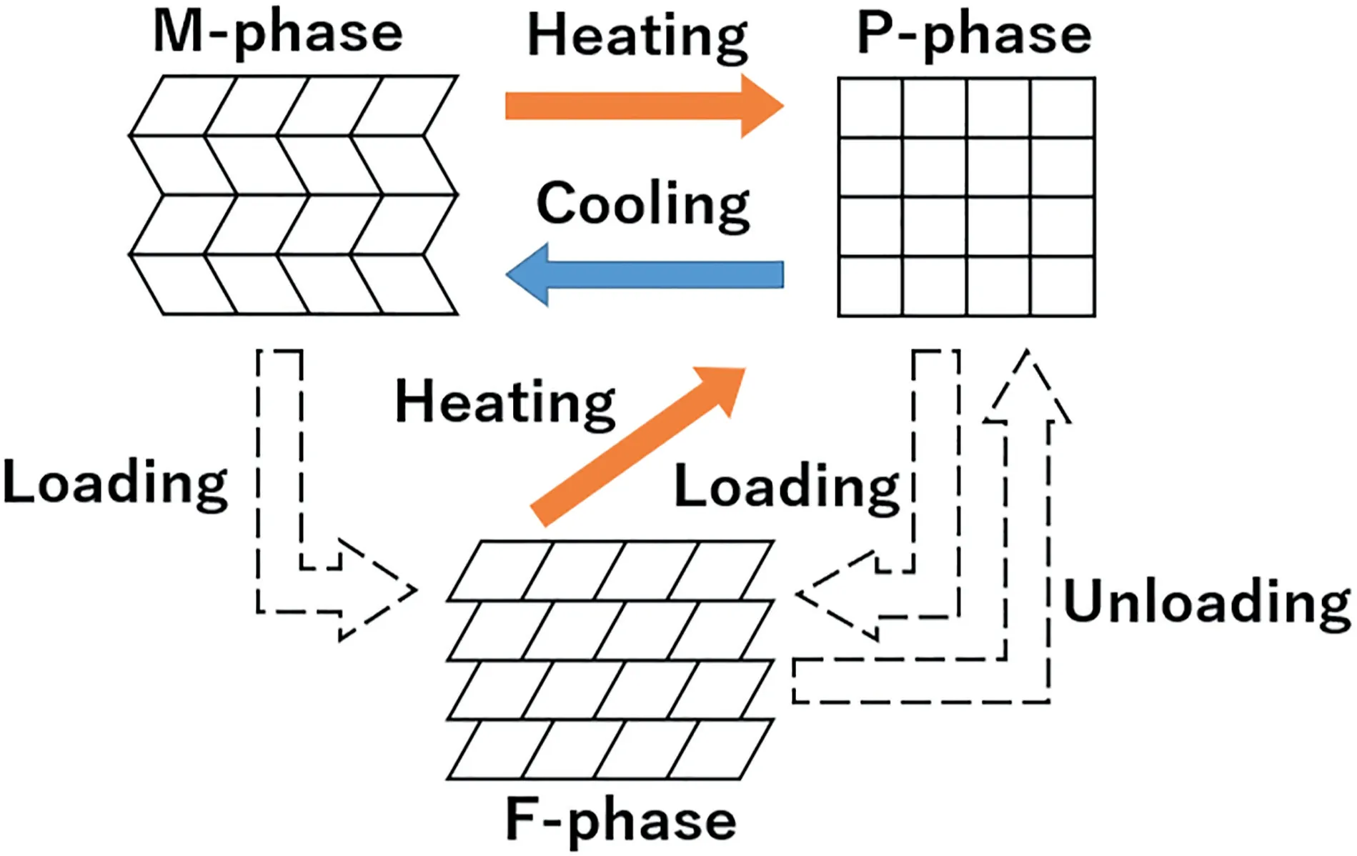
FIGURE 1 Three‐phase transformation in shape memory alloy(SMA)
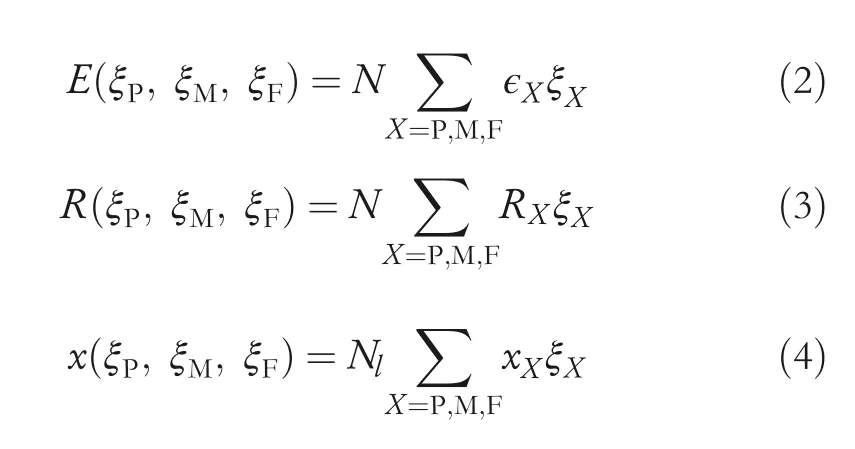
In those equations,Ndenotes the total number of unit lattice andNlstands for the number of unit lattice in longitudinal distance.Also,ϵP,ϵMandϵFrepresent the internal energy,RP,RMandRFare resistance values,andxP,xMandxFrepresent the longitudinal distances per unit lattice of the P,M,and F phases.The total numberNis

whereNA(mol−1)is Avogadro's constant,x0(m)denotes the length of the SMA at low temperature and no load,and no load has been applied in the past.ρL(kg/m)stands for line density,θdenotes the ratio ofTiin SMA.Also,ATiandANi,respectively,express the molar masses ofTiandNi.The total number of unit latticeNis defined as half the number of atoms of SMA because there are two atoms per unit lattice of the P‐phase.Ncan also be expressed as follows.
whereNSrepresents the number of unit lattice on short direction.It is assumed that the crystal lattice of P‐phase is perfect cubic.The volume and cross‐sectional area per unit lattice of the A‐phase can be represented asN(xP)3(m3)andNS(xP)2(m2).For that reason,the relation between the volume,cross‐sectional area,length and the number of unit lattice can be described as shown below.
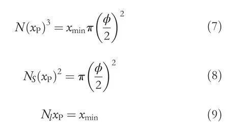
Therein,ϕ(m)denotes the diameter of the cross section;the diameterϕis assumed to be a constant.xmin(m)expresses the length of SMA when all crystal lattices are P‐phase.
Next,the entropySC(J/K)of SMA is derived.Shape memory alloy undergoes a phase transformation under external stimuli,and it is assumed that a complex combination of P,M,and F phases exists randomly during the phase transformation.Then,entropySCcan be defined as

wherekB(J/K)is Boltzmann's constant.
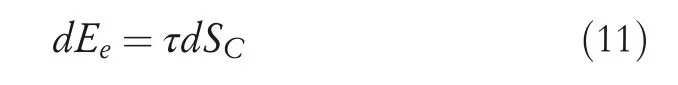
When several phases are mixed inside SMA,elastic interaction energy between the different phases occurs[26].Calculating the elastic interaction energy from a micro perspective requires an enormous amount of calculation.It is therefore unsuitable as a mathematical model for real‐time processing when integrated into an actual control system.Therefore,the elastic interaction energy is represented by an expression that is as simplified as possible.The minute change in the elastic interaction energy of the SMA,dEe(J),is attributable to the change in the misfit between the different phases.It can be regarded as proportional todSC,which represents mixing of the P,M,and F phase.Then,the elastic interaction energy is defined as

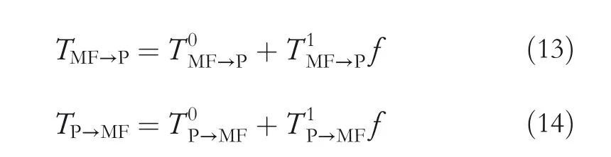
whereτ(°C)can be approximated by phase transformation temperatures as where sgn(˙T)represents the sign function of the time derivative of temperatureT,which extracts the sign of the rise and fall in temperature.Also,TMF→Pis the phase transformation temperature from the mixed phase of M and F phases to P‐phase.In addition,TP→MFis the phase transformation from P‐phase to the mixed phase of M and F phases.TMF→PandTP→MFcan be represented as a linear function of the loadf(kg)such that
2.3|Energy balance of shape memory alloy
Based on the first law of thermodynamics,the equation in terms of energy balance of SMA is derived.The thermal energy TdSC(J),which denotes the quantity of energy supplied at heat is obtained as

wheredE(J)is the change in internal energy anddW(J)is the work done to its surroundings,which is reversible at a temperature where SE occurs,and which is irreversible at lower temperatures.The strain caused by irreversible work is recovered by heating.When SMA undergoes a phase transformation because of SE or SME,dWcan be defined asdW=fdx.The derivatives of internal energyE,lengthx,and entropySCare presented below.
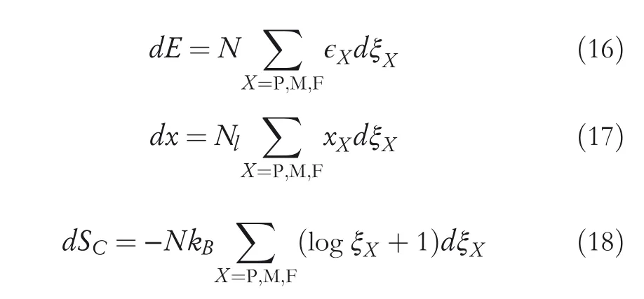
One can substitute Equations(6),(11)and(16)–(18)into(15),then arrange(15)by the derivative of the fractionξP,ξMandξF.
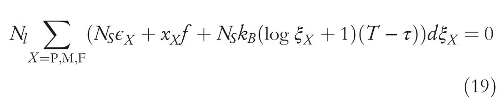
Solving Equation(19)requires the calculation of derivatives∂ξX/∂ξY(X,Y=P,M,F)with respect toξP,ξMandξF.It can be determined from lattice structure of each phase.The derivatives are defined as
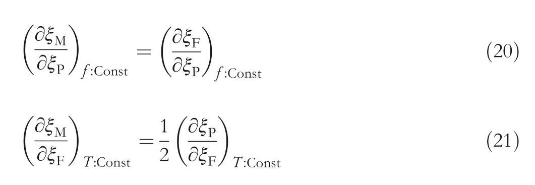
wheref:Const andT:Const,respectively,represent load and Temperature are constants.Because the phase transformation from M‐phase to F‐phase is irreversible,Equation(21)only holds when F‐phase increases.
2.4|Mathematical model under a constant load
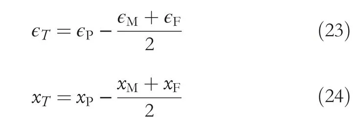
From Equations(19)and(20),the model under the constant loaddf=0 can be derived as
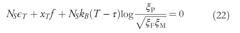
where constantsϵT(J)andxT(m)are as presented below.
When the SMA temperature rises,P‐phase increases and M‐phase and F‐phase decrease.In the presence of a loadf,F‐phase remains even at high temperature.When the SMA with a loadfis heated sufficiently,the amount of remaining F‐phase can be represented asξFmin(f).Actually,ξFmin(f)is the minimum value of F‐phase with loadf.When no load is applied and SMA is completely in P‐phase,ξFmin(f)=0.The fractionξFis defined as presented below.

When the loadfis a constant,ξFmin(f)is a constant anddξ′Fis a variable.From Equation(20),it is apparent that the fractions ofξMandξFare the same amount.Among the minute changes in the fraction of P,M and F phases,the following relation holds.
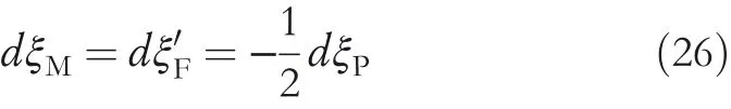
Therein,the mixed phase of M and F phases,ξMF,is defined as the following equation.
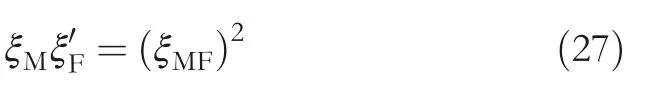
Substituting Equations(25)and(27)into(22),one obtainsξFandξMFunder a constant load as

By substituting Equations(28)and(29)into(3),one can obtain the resistance model under a constant load as

In addition,a temperature sensing model under a constant load is calculated by solving Equation(30)for temperatureT.
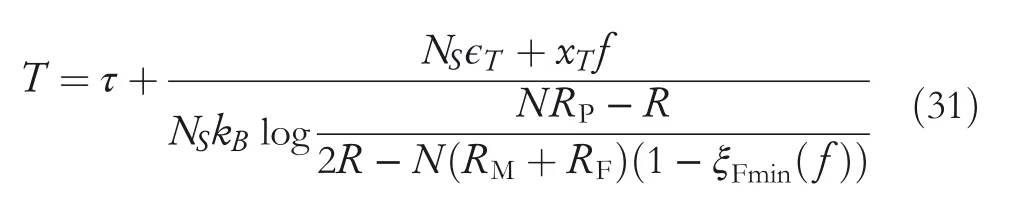
The temperature sensing model is useful as a compensator for non‐linear characteristics of an SMA actuator.
2.5|Mathematical model under a constant temperature
From Equations(19)and(21),the model under the constant temperaturedT=0 can be derived as shown below.
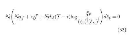
Therein,the constantsϵf(J)andxf(m)are as defined below.

From Equation(32),the fraction of the crystal latticeξP,ξMandξFunder a constant temperature is obtainable as presented in the equations below.
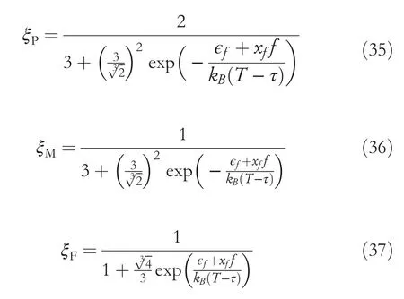
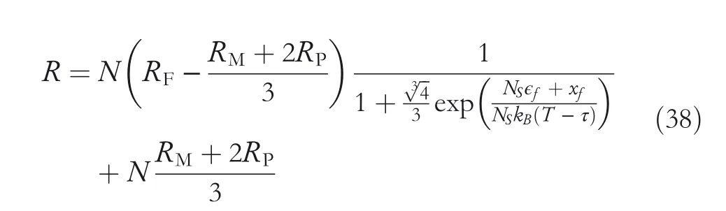
Therefore,the resistance model under a constant temperature is
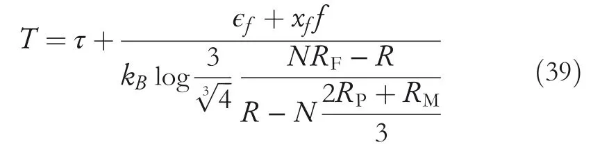
Additionally,the temperature sensing model under constant temperature is calculated by solving Equation(38)for temperatureT.
3|PARAMETER IDENTIFICATION AND MODEL VALIDATION
Some model parameters such as the number of crystal lattices and values per unit lattice of P‐phase are obtained from physical properties.Table 1 presents the model parameters.We assumed the ratio ofTiin SMA asθ=0.5 because it is not P‐phase at room temperature.When heated sufficiently with no load,the length of SMA,xmin(m),was 0.782 m.NS,Nl,N,andxPwere calculated using Equations(5 and 7–9).Earlier research reports describe the longitudinal distance per unit lattice of the P,xP,as approximately 3.010~3.020Å,closely approximating the obtained value ofxP=3.0107Å.
3.1|Experimental environment
The relation between resistance,load,and temperature was investigated by temperature experiments conducted with a thermostat chamber.The experiments used Ti–Ni SMA wire(BMF150;Toki Corp.)with dimensions of 0.15 mm diameter and 0.800 m length at room temperature and zero load.Because SMA undergoes a phase transformation under two external stimuli,experiments were conducted separately under a constant load and a constant temperature.This study only considered the load on longitudinal direction of SMA wire,not the load on the short direction.
Figure 2 portrays an outline of an experiment setup,and the photo of the experimental setup are shown in Figure 3.For the experiment under a constant load(Figure 2a),the temperature inside the chamber was varied,whereas a constant weight was loaded on the SMA wire.The temperature and the electrical resistance values were observed using a temperature sensor and a digital multimeter.On the other hand,for theexperiment under a constant temperature(Figure 2b),the SMA wire inside the chamber was connected to a force meter mounted on theXaxis stage.The electrical resistance and the load were observed as the stage moved in the longitudinal direction of the SMA.
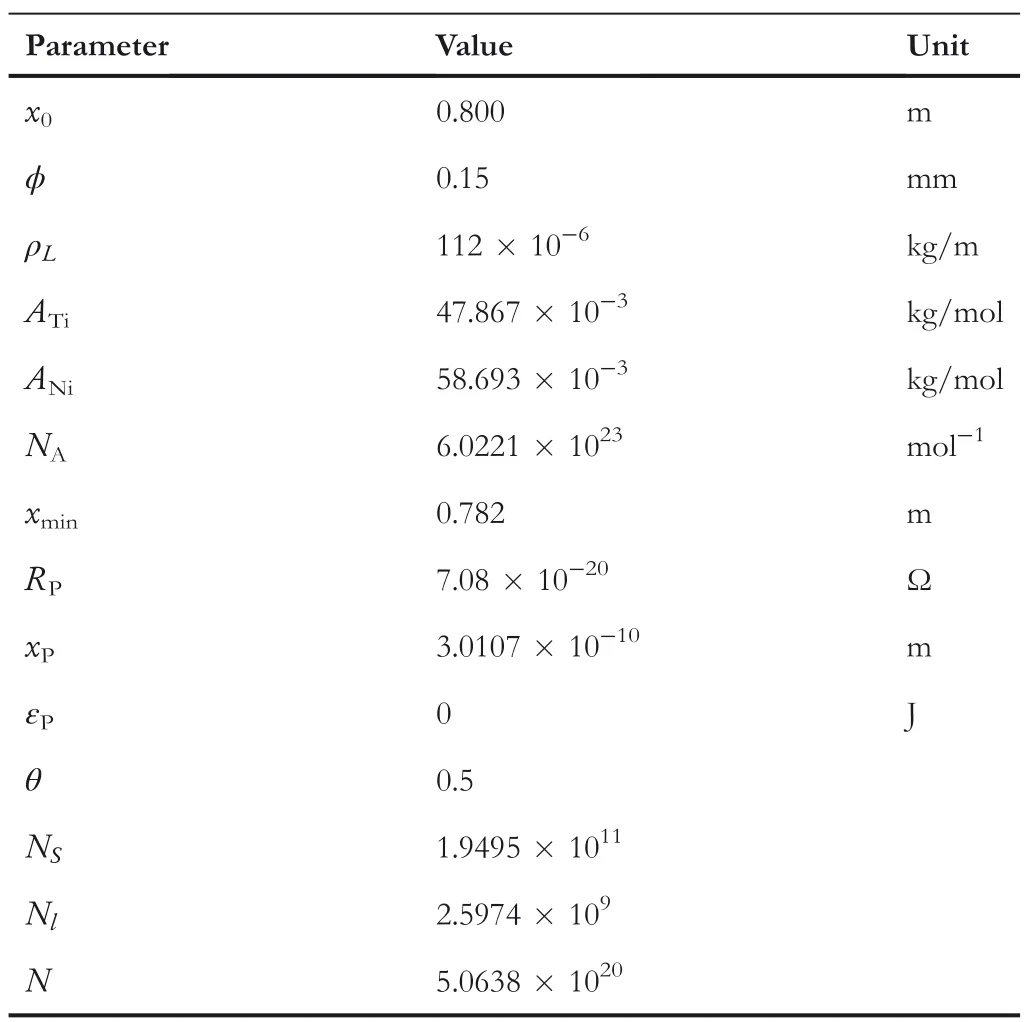
TABLE 1 Crystal lattice and P‐phase related parameters
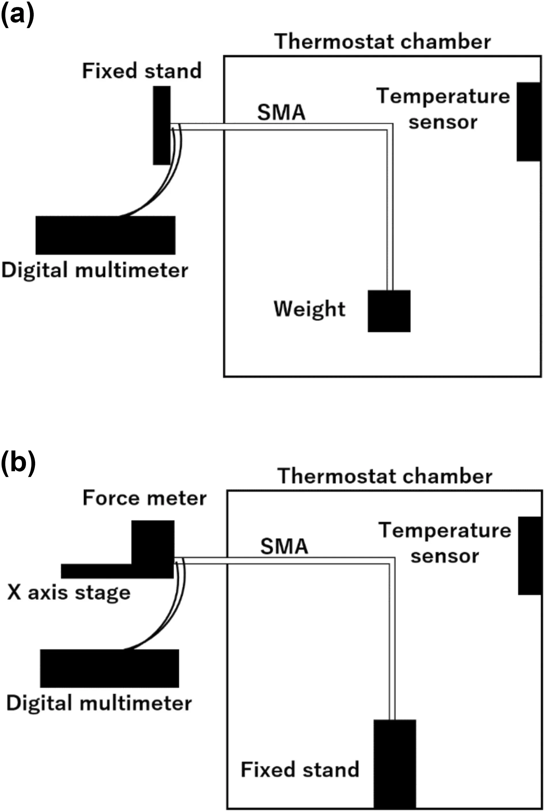
FIGURE 2 Outline of experimental setup for load,electrical resistance,and temperature measurement.(a)Experiment under a constant load.(b)Experiment under a constant temperature
3.2|Comparison of temperature—electrical resistance characteristics
To identify parameters of the resistance model represented by Equation(30),the relation between the SMA wire temperature and the electrical resistance was investigated by varying the internal temperature of the thermostat chamber.The chamber temperature was varied in sufficient time that can be regarded as equal to the internal temperature of the SMA wire.The measurement temperatures were from 10 to 110°C.The loads in the experiments were determined by considering the practical force produced(1.50×10⁻¹kg),and comparisons between mathematical model and experimental results were made with several weights ranging from 3.2×10⁻³to 1.50×10⁻¹kg.This chapter presents comparisons when hanging 0.50×10⁻¹and 1.50×10⁻¹kg weights on the SMA wire.The experimentally obtained results portrayed in Figure 4 were measured electrical resistance values at varying temperatures.Table 2 presents the mathematical model parameters,which were determined so that the mean absolute percentage error between the model and experimentally obtained data was less than 3.0%.As the load increases,the hysteresis width increases and the phase transition temperature shifts to a higher temperature.Although complex non‐linear characteristics such as hysteresis and saturation are visible in Figure 4,it is apparent that the mathematical model shows good agreement with the experimentally obtained data.
3.3|Comparison between the temperature sensing model and experiment results
The temperature sensing model represented by Equation(31)was compared to experimentally obtained data.The data portrayed in Figure 5 show that the input is electrical resistance and that the output is temperature.That is,the figure is an inversion of the input and output relation depicted in Figure 4.In Figure 5,the temperature sensing model and experimentally obtained data show good agreement over the range where SMA is undergoing a phase transformation.In contrast,the temperature is not sensed correctly over the area where the electrical resistance is saturated.The temperature sensing model is only valid while SMA is in a phase transformation.Therefore,the temperature cannot be sensed in the section where resistance is saturated.
3.4|Comparison of load—electrical resistance characteristics
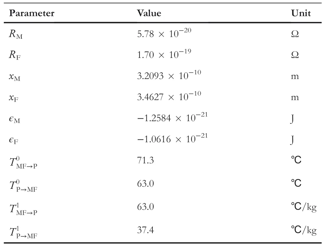
TABLE 2 Identified model parameters
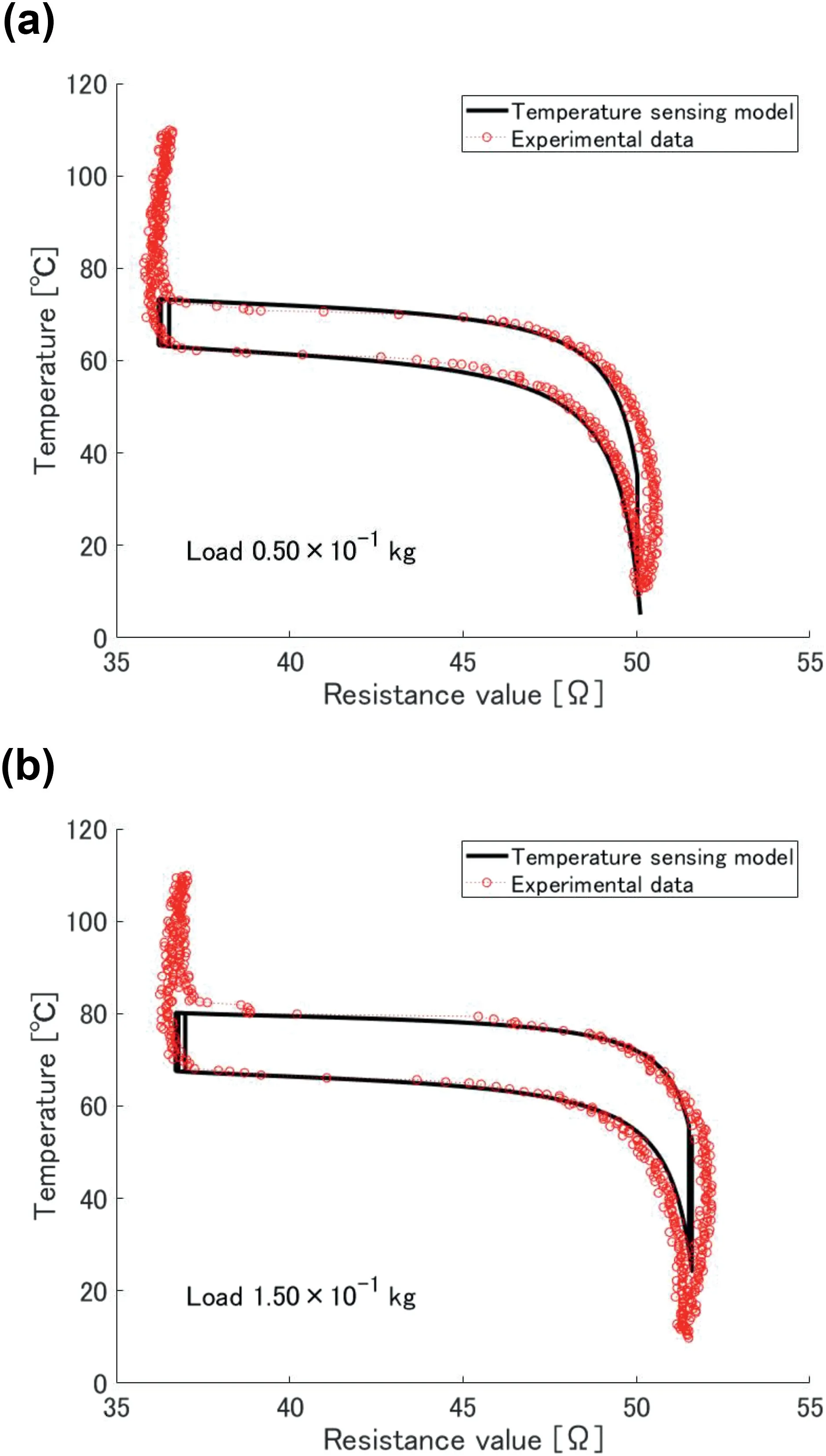
FIGURE 5 Comparison between temperature sensing model and experiment results.(a)Constant load:0.50×10⁻¹ kg.(b)Constant load:1.50×10⁻¹ kg
The resistance model under a constant temperature represented by Equation(38)was compared to experimentally obtained data.As described in Section 2.1,when stress is applied to M‐phase at low temperature,stress‐induced martensitic phase transformation occurs,and F‐phase does not reverse to M‐phase even if stress decreases.To verify if the model can represent the transformation at low temperature,while maintaining the SMA temperature at the constant value of 20.0°C,the relation between load and electrical resistance was investigated by varying the load.The resistance values when varying the load are presented in Figure 6.Experiment results indicate that after the load was increased to 0.1 kg,it decreased to less than 0.03 kg.Subsequently,0.2 and 0.3 kg decreased similarly.The result in Figure 6 suggests the model can represent the change in electrical resistance during stress‐induced martensitic phase transformation.
3.5|Consideration of a mathematical model under constant shape memory alloy length
To evaluate whether the proposed mathematical model can be represented accurately at arbitrary change in temperature and load,an experiment was conducted under a constant length,varying load,and temperature.For the experiment,the SMA wire was fixed at an initial length of 0.80 m,which is the length at low temperature and no load.No load has been applied in the past.The experiment used the setup presented in Figure 3.Then,the load varied by the temperature rise of SMA was measured.
By solving Equation(19)under a constant length,a relational expression between temperature and load can be derived.From Maxwell relations,relation on the variation of load and temperature holds.

In Equation(40),the left side represents the slope in the temperature—load plane.The right side represents the ratio between entropy and length changes under a constant temperature.The derivative of lengthx,dx,can be written as
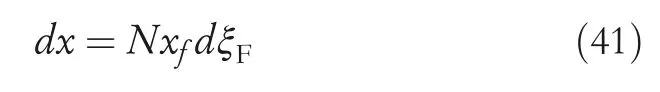
wherexfis the constant defined by Equation(34).One can substitute Equation(41)into the right side of Equation(40).

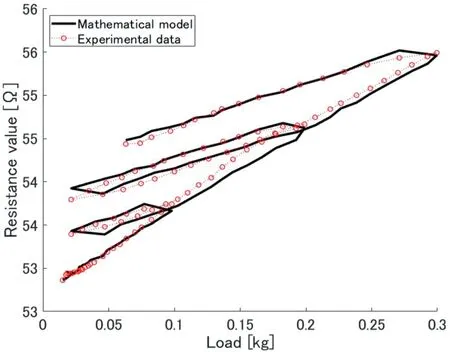
FIGURE 6 Load—electrical resistance characteristics at constant temperature(20.0°C)
Therein,it is assumed that no phase transformation occurs when the SMA wire length is a constant,the right side is a constant.Equation(40)shows that an SMA fixed at a constant length exhibits linear characteristics in the temperature—load plane.Equation(42)depends on the fraction of the crystal lattice of SMAξP,ξMandξF.The value is calculated by the fraction on the initial length.From the experimentally obtained result,ξP=0.4391,ξF=0.2805,andξM=0.2805 were obtained.Substituting the fraction into Equation(42),it can be obtained as(∂f/∂T)x=9.945×10−3kg/K.The experimentally obtained result of temperature–load characteristics is depicted in Figure 7,where the solid line represents the simulation result,and the red dotted line represents experimentally obtained data.Figure 7 shows that the experimentally obtained result and simulation result agree well at temperatures higher than 60.0°C.However,a large discrepancy exists below 60.0°C.That outcome was expected because little load was applied to the SMA wire while the wire was sagging.
4|SIMULATION RESULTS OF AN ELECTRICAL RESISTANCE CONTROL SYSTEM
In this section,the effectiveness of the proposed model as a non‐linear compensator is confirmed by numerical simulations.An electrical resistance control system using classic feedback–feedforward control method is employed to validate the compensator.In general,SMA actuators represent hysteresis and heat transfer characteristics that can be defined by the first‐order dynamic equation.The feedforward controller has a function of hysteresis compensation and response improvement due to the heat transfer characteristics.
4.1|Shape memory alloy actuator model
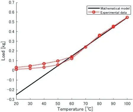
FIGURE 7 Temperature—Load characteristics under a constant length
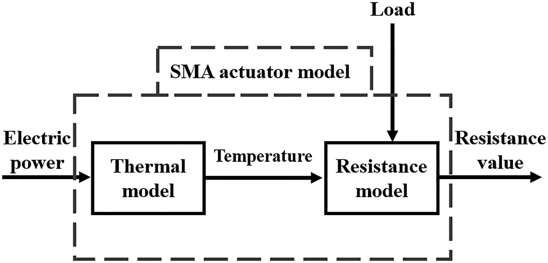
FIGURE 8 Shape memory alloy(SMA)actuator model
An SMA wire is considered as an SMA actuator to be modelled.A simplified block diagram of the SMA actuator model is portrayed in Figure 8.The block diagram is divided into two parts:Thermal model and Resistance model.Resistance model used the mathematical model of Equation(30).In Thermal model,the input is electric power,which is characterised electric current.The model output is temperature.Thermal model is defined by the heat transfer equation,where it is assumed that heat loss occurs only via natural convection.The temperature dynamics are given by the following differential equation[27,28]as
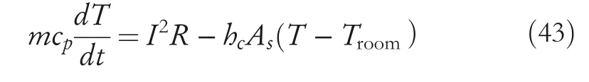
whereI(A)stands for the electric current,As(m2)denotes the surface area,cp(J/kg°C)signifies the specific heat,m(kg)expresses the mass,hc(W/m2°C)represents the heat convection coefficient,andTroom(°C)is the ambient temperature.Although the wire surface area will change during the SMA actuator operation,it is assumed that these effects are negligible.The thermal model parameters are given asAs=3.77×10⁻⁴m2,cp=465 J/kg°C,m=89.6×10−6kg,hc=106 W/m2°C,andTroom=10°C.
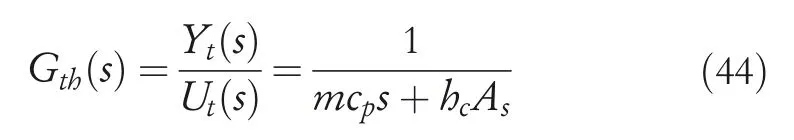
For convenience,the electric powerI2Rand the difference in temperatureT−Troomare defined asutandyt.We assumed that Thermal model can be considered as first‐order lag system.Then,Transfer function of Thermal modelGthcan be presented below.
4.2|Electrical resistance control system
The outline of the electrical resistance control system using the proposed temperature sensing model is presented in Figure 9.Load represents the weight suspended on an SMA wire,for which the weight changes during operation.Presumably,the load fluctuation is obtainable using physical sensors such as load cell.The load weight is input into the temperature sensing model.The non‐linear characteristics of SMA are compensated by the temperature sensing model represented by Equation(31).The output of the temperature sensing model varies rapidly when the electrical resistance is saturated,and the rapid change can affect the control performance of the system.Therefore,Phase‐lag compensatorCplwas designed to reduce the influence of the rapid change,and the compensator also can compensate for delay in heat transfer process.The compensatorCpl(s)is defined as
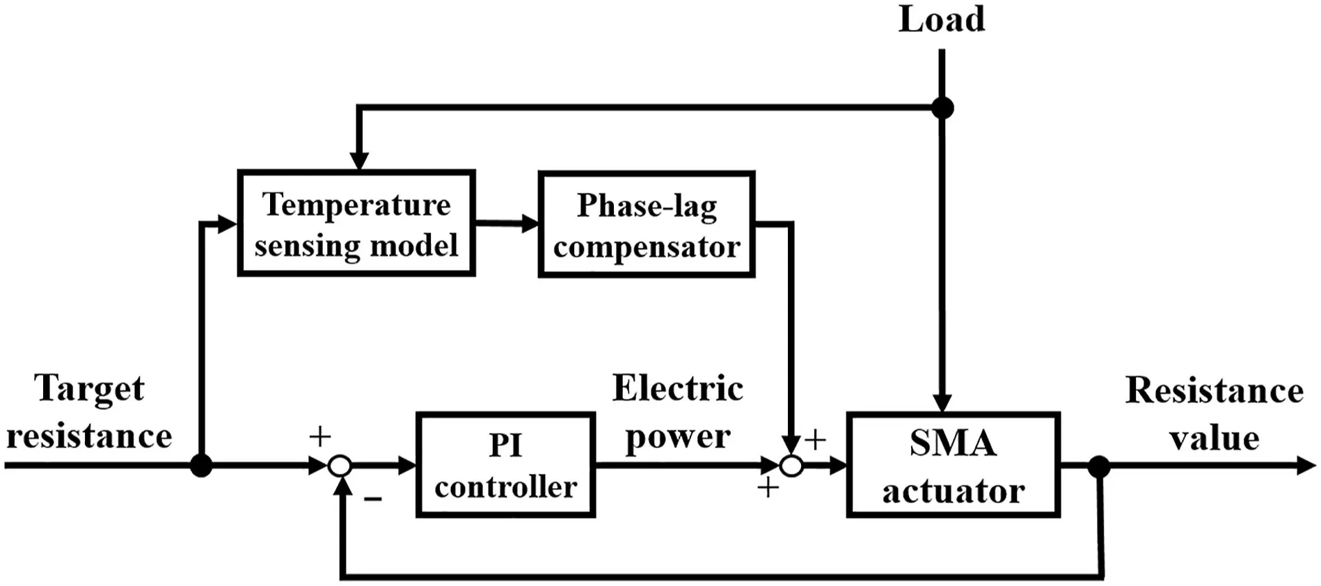
FIGURE 9 Block diagram of the electrical resistance control system
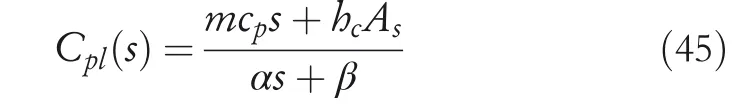
The parametersαandβwere defined by trial and error.The feedback control with PI controller can eliminate the error of the electrical resistance,and plays a supporting function in this system.
4.3|Numerical simulation results
Figure 10 presents the simulation results obtained from tracking a 0.5 Hz sinusoidal signal using the resistance control system shown in Figure 9.In the graph above,the blue broken line represents a load,where the load was varied every 10 s,which 3.2×10⁻³kg was applied att<10 s,0.50×10−1kg at 10 s≤t<20 s,and 1.50×10⁻¹kg att≥20 s.The black line represents input power.The input power to the SMA actuator was limited so that 0 W or less is 0 W in the simulations.In the graph below,the black broken line represents the reference input.The reference trajectoryxrefwas calculated as shown below.
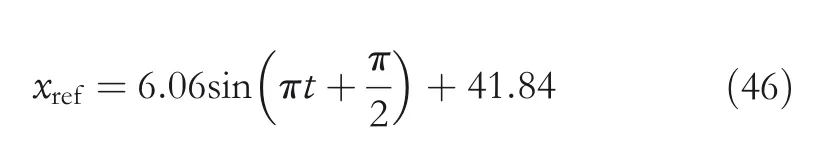
In that equation,the reference value is the target resistance,which varies in the range of phase transformation,ranging from 35.8 to 47.9 Ω.The red line represents the output of the system,which is the electrical resistance of the SMA actuator.
Figure 10a shows the result without the feedforward compensator.In Figure 10b,c,the feedforward compensators based on the temperature sensing model were used.Figure 10b used the temperature sensing model under a constant load(0.50×10⁻¹kg).The model does not take into account load variation,in other words,it is the model in which the input is resistance and the output is temperature under a constant load.By contrast,Figure 10c used the temperature sensing model adapting to load fluctuation.For the entire simulation,the gains of the PI controller used same values.The parameters used in the PI controller and Phase‐lag compensator shown in Equation(42)are listed in Table 3.The tracking errors of Figure 10a are large compared with the results of compensators shown in Figure 10b,c.This findings can be attributed mainly to the non‐linear characteristics of SMA.However,Figure 10b,c show that the feedforward compensator based on temperature sensing model achieves better tracking response.The shape of the input powers with feedforward compensators shown in Figure 10b,c differ from the input power with PI control shown in Figure 10a around the value at which the electrical resistance saturates.In Figure 10b,c,either input power and output resistance show no significant difference.
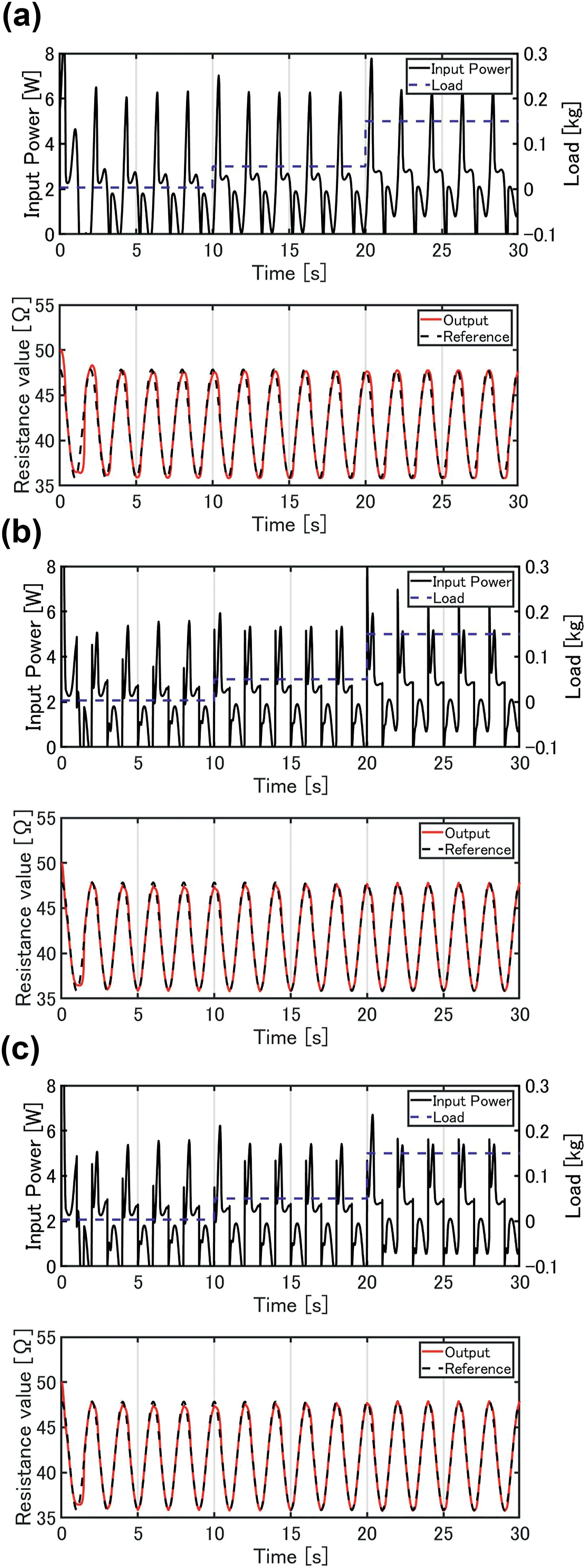
FIGURE 1 0 Numerical simulation results of tracking a sinusoidal signal.(a)PI control.(b)PI control+Temperature sensing model unadapted to load fluctuation.(c)PI control+Temperature sensing model adapting to load fluctuation
The model used in Figure 10b was designed with a constant load(0.50×10⁻¹kg),the greater the difference between the load applied to the SMA actuator,the greater effect on tracking performance.To confirm the effect on tracking performance,simulation was performed under a constant load(2.50×10⁻¹kg).An enlarged view of three outputs is shown in Figure 11.PI control alone shows slow response because the control input remains small until exiting the saturation region of hysteresis.In addition,even when the reference input is varying almost linearly,the system is also affected by the non‐linear characteristics.On the other hand,the results obtained using the temperature sensing model show good tracking performance.It is because that the shape of the hysteresis does not change with a load significantly,an accurate inverse model of hysteresis can compensate for non‐linear characteristics even in the presence of load fluctuation to some extent.However,as a load increases,the phase transformationtemperature of SMA shifts to the high temperature side and the hysteresis width also increases.As a result,the control input when not adapting to load fluctuation cannot be applied at the proper timing and the tracking performance is a little poor as shown in Figure 11.It is apparent that the control system with a compensator adapting to load fluctuation follows the reference with better accuracy than the others.Consequently,the proposed hysteresis model proves to be effective for non‐linear compensation of the resistance control system adapting to load fluctuation of the SMA actuator.
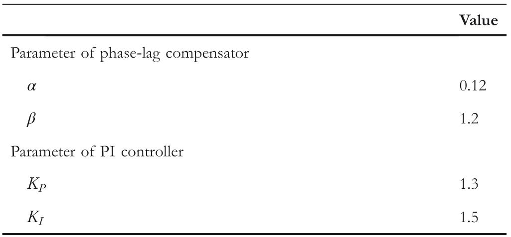
TABLE 3 Parameters of phase‐lag compensator and PI controller
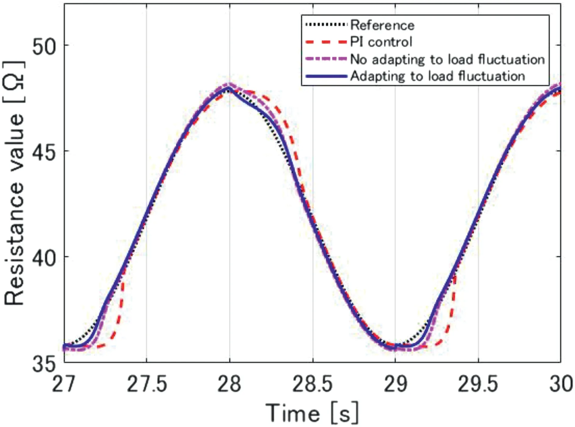
FIGURE 1 1 Comparison of three outputs
5|CONCLUSION
In this study,we showed a new approach to construct a hysteresis mathematical model of an SMA actuator based on the laws of thermodynamics.The hysteresis model takes into account load fluctuation,and besides,the inverse model used for non‐linear characteristics compensation of SMA can simply be designed by the hysteresis model.The model validation was examined through the comparison to experimental results;the proposed model was able to represent complex non‐linearities of SMA with the mean absolute percentage error of less than 3.0%.In addition,we successfully applied the model to the compensator of an electrical resistance control system,with the simulation results providing its advantages.However,a problem remains unsolved.When the resistance is saturated,the model cannot represent the non‐linear characteristics of SMA.If the model could represent saturated region,we could achieve smooth control.In future,it would be interesting to extend to the strain control system using the proposed hysteresis model considering load fluctuation and we will implement experiments.
DATA AVAILABILITY STATEMENT
The datasets generated and/or analyzed during the current study are available from the corresponding author on reasonable request.
ORCID
Seiji Saitohttps://orcid.org/0000-0002-5874-776X
杂志排行

CAAI Transactions on Intelligence Technology的其它文章
- Apple grading method based on neural network with ordered partitions and evidential ensemble learning
- An improved bearing fault detection strategy based on artificial bee colony algorithm
- Parameter optimization of control system design for uncertain wireless power transfer systems using modified genetic algorithm
- Passive robust control for uncertain Hamiltonian systems by using operator theory
- Humanoid control of lower limb exoskeleton robot based on human gait data with sliding mode neural network
- Research on trend prediction of component stock in fuzzy time series based on deep forest