Realizing number recognition with simulated quantum semi-restricted Boltzmann machine
2022-10-22FuwenZhangYonggangTanandQingyuCai
Fuwen Zhang,Yonggang Tan and Qing-yu Cai
1 School of Physics,Zhengzhou University,Zhengzhou 450001,China
2 Innovation Academy for Precision Measurement Science and Technology,Chinese Academy of Sciences,Wuhan 430071,China
3 School of Physics and Electronic Information,Luoyang Normal University,Luoyang 471934,China
4 Center for Theoretical physics,Hainan University,Haikou 570228,China
5 School of Information and Communication Engineering,Hainan University,Haikou 570228,China
Abstract Quantum machine learning based on quantum algorithms may achieve an exponential speedup over classical algorithms in dealing with some problems such as clustering.In this paper,we use the method of training the lower bound of the average log likelihood function on the quantum Boltzmann machine (QBM) to recognize the handwritten number datasets and compare the training results with classical models.We find that,when the QBM is semi-restricted,the training results get better with fewer computing resources.This shows that it is necessary to design a targeted algorithm to speed up computation and save resources.
Keywords: machine learning,quantum Boltzmann machine,quantum algorithm
1.Introduction
The Boltzmann machine (BM) [1]is an undirected model consisting of visible layers and hidden layers.The information is input from the visible layer and obeys the Boltzmann distribution in the hidden layer.It has been widely applied in many fields,such as phone recognition tasks [2],image recognition [3],medical health [4],the quantum many-body problem [5],and so on.In BM training,it is difficult to compute the negative phase value of the partial derivative of the average likelihood function,since its computational complexity will increase exponentially with the dimensions and the quantity of the training data.This difficulty can be solved by using Gibbs sampling to gain the expectations of the computational model.
The mixing of the Gibbs sampler becomes slow when the sampling data are complicated.Hinton proposed the contrast divergence (CD) method [6]to solve the slow sampling problem.The method assumes that there is a fantasy particle,and N steps of Gibbs sampling at the fantasy particle are run to replace the model distribution.The CD method performs well in actual training [7].Alternatively,there is another technique to solve the model expectation named the persistent comparison divergence (PCD).The procedure is that when the state stof the fantasy particle and the corresponding parameter θtare known at time t,one can get st+δtat the time t+δt by transferring the operator.Then the parameters of the model are updated to the parameter θt+δtat the time t+δt.Different from the CD method,it requires reducing the learning rate with the update to ensure the convergence of the model [8].Deep belief networks [9]and deep BMs [10]can be obtained by using the stack of BM,the training of which could be done with the greedy layerwise strategy.The greedy layerwise strategy contains the process of pre-training the model,which is more efficient than the random selection of parameters.The deep model [11]can learn the deep patterns and the abstract concepts of data,which has great advantages over the shallow learning in learning and interpreting complicated data [12].

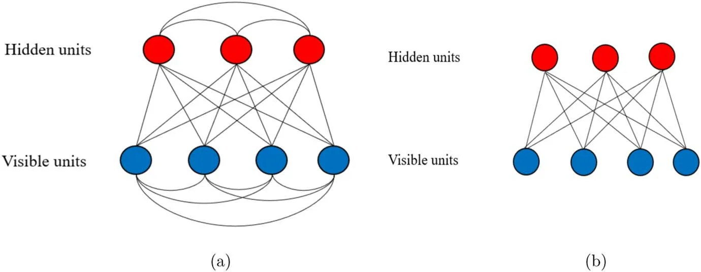
Figure 1.(a) The model of fully connected BM.The blue circles represent visible units,and the red circles represent hidden units.(b) The model of RBM without lateral connectivity both in the visible units and in the hidden units.
In practice,the dimensions and quantity of some tasks,such as computer version [13],and speech recognition [14],are usually huge,training of which requires huge computing resources.If these tasks are performed in the classical way,there are disadvantages such as slow training speed and easily falling into local minima [15].In order to overcome these shortcomings,scientists proposed to optimize classical machine learning algorithms by exploiting the potential of quantum computing[16].The combination of quantum theory with BM is generally called quantum Boltzmann machine(QBM)which can be mainly divided into two directions,one is based on the quantum variational principle method [17],and the other is based on the quantum annealing method[18].
In the quantum variational principle method,the Gibbs state for a given Hamiltonian is approximately generated by combining the quantum approximate optimization algorithm or the variational quantum imaginary time evolution algorithm,and then the parameters can be adjusted [19,20].The quantum annealing algorithm is based on the principle of the quantum tunneling effect[21].Under the annealing condition,the quantum configuration energy will eventually evolve into the ground state and the training parameters are in the global optimal solution.Usually,annealing can be realized by using quantum annealing machines to construct a QBM model.Quantum annealing methods outperform classical methods in a number of iterations when recognizing numerical tasks[22].
The purpose of this paper is to demonstrate the possibility of digit recognition with various QBMs,particularly the quantum semi-restricted Boltzmann machines(QSRBM).We train the dataset on a QSRBM based on the method of training the lower bound of the quantum log likelihood function and give the training fidelity.This paper is organized as follows.In the second section,the principle of BM and QBM is briefly introduced.Then we show the processing of training data and the results of training.Finally,we discuss and conclude.
2.Quantum BM
BM in figure 1 (a) can be changed into various machines by adjusting the connection of layers.One can get a restricted Boltzmann machine (RBM) by disconnecting the lateral connectivity in the BM.QBM can be constructed by replacing the data units with corresponding operators.
2.1.Restricted BM
BM is a fully connected model including the lateral connection in the layers,which may cause additional computational complexity when dealing with some problems.As an improvement in some cases,there is no such connection in the layers of RBM.Without affecting the training performance,the RBM model is simpler and more efficient [23]and has been applied to some practical problems[24,25].The energy function of the joint configuration of RBM is given by

where viis the binary state of the visible unit i,hjis the binary state of the hidden unit j,ai,bj,wijare the connection strengths between the unit layers,and θ ∈ai,bj,wij[26].The probability distribution of the visible unit is [27]

where Z is the partition function.The machine with connections in figure 1(b)is called RBM[28],and the hidden units of RBM are independent of given visible units.The expected value of the data can be obtained in only one parallel step,thus greatly reducing the amount of computation [27].
Usually,the training process can be performed by minimizing the negative average log likelihood function ζ

The parameters can be trained by taking partial derivatives of the likelihood function

with the gradient descent algorithm [29]

where η is the learning rate.η needs to be selected according to the actual problem: If η is too large,it is easy to miss the best solution,resulting in divergence;If η is too small,the number of the iteration steps will be too large.In equation(5),〈v〉dataare the clamped expectation with v fixed,which can be easily calculated by Gibbs sampling.〈v〉modelare the expected value of v over the model probability distribution,the calculation of 〈v〉modelrequires solving the value of the partition function Z and the parameters of the BM,which is almost incalculable and uneconomical for complicated data.The partial derivative of the negative log likelihood function can often be approximated by CD method,which uses the sampling formula [30]

to sample the data.By sampling the data n times,the update rules in equation (5) are changed into

The update rules which respect to the weights ai,bjare similar to equation (7).Even taking n=1,the CD method usually works well [7].
2.2.QBM and quantum semi-restricted BM
QBM can be obtained by a quantum approximate optimization algorithm method [31].Alternatively,it can be constructed QBM by mapping the units of BM to the qubits of the D-Wave system [32]that exploits the advantage of quantum tunneling.One can use variational quantum imaginary time evolution to obtain the Gibbs state of the QBM model and realize training [19].One can also use the model whose visible layers are still classical and only change the hidden layers from classical variables to a quantum degree of freedom,which can be trained with the PCD method [33].
For simplicity,the Hamiltonian H of a QBM model is given by [34]

where

and I and σzare the identity operator and Pauli operator respectively.The classical p(v) in equation (2) can be obtained by tracing the hidden unit of the density matrix ρ on the QBM

where Λv=|v〉〈v|⊗Ih.Then the equation(4)is replaced with

The first term on the right side in equation (11) cannot be directly processed for derivation.This problem can be solved by finding the upper bound with Golden–Thompson inequality [35]

Setting

we have that
and then

Minimizing the upper bound ζupof ζ,one can obtain

Since the fully connected QBM is too complicated,for simplicity,we consider disconnecting the connection in the hidden layers,the quantum version of which is usually called QSRBM.The Hamiltonian in equation(13)can hence be rewritten as

where ciis the connection strength within visible layers,fie=ai+∑μ wiμ vμ,and

Combining equation (11) and equation (17),one can get


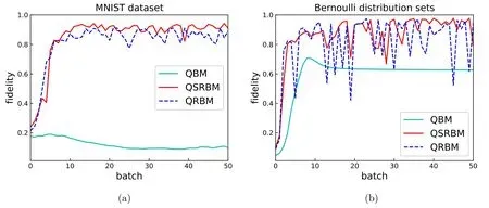
Figure 2.(a)The training of MNIST datasets in QBM,QRBM and QSRBM.The accuracy rate of MNIST datasets reaches to 0.109,0.845,0.942 respectively,when the number of batches is 49.(b) The training of Bernoulli distribution sets in QBM,QRBM and QSRBM.The accuracy rate of Bernoulli distribution sets reaches to 0.627,0.618,0.977 respectively,when the number of batch is 49.
3.Training results
We firstly process the data to fit our models and then give the training results.Our results show that the recognition rate of the quantum algorithm can be close to the classical results even with small resources.
3.1.Data processing
For Bernoulli distribution,we use

to generate a set of binary data.Here,p,q are the probability of generating 1,0 each time,p=1-q,n is the trial count,and x is the sum of the generating number.f(x|p)is the probability of obtaining x after the n trials.We set p=0.9 here(We also trained the machines with other values of p).
The MNIST dataset was first introduced by LeCun et al[37].It is an optical pixel set of 10 Arabic numerals,containing a total of 70 000 images with a resolution 28×28.Since the outer pixel value of the most of dataset is 0,we firstly eliminated the outer 2 pixels,and hence the pixels are reduced to 24×24 size.Next,every 8×8 pixel value is averaged to reduce the digital image to 3×3 pixels.Although 3×3 pixels could not be used to distinguish digital with our naked eyes,they still contain most of the information of digital images and are representative.The times of iterations on training Bernoulli distribution sets and MNIST dataset with RBM are 1000 and 30 000,respectively.The Bernoulli distribution sets and MNIST dataset are trained by using fully connected QBM,RBM,QRBM and QSRBM,respectively.The number of visible and hidden units here is 9 and 2,respectively.
An important improvement on the original model [34]is converting the measurement of work performance from Kullback–Leibler divergence [38]value to the fidelity betweenpvdataand pv.It will make our training results have an intuitive comparison with other types of QBM,the classical BM,and other models of the same data type training.The fidelity is given by

wherepvdatais the probability distribution of training data.
3.2.Simulation conditions
The CPU of our computer is Intel 8 cores and its model is Intel(R) Xeon(R) CPU E3-1245 v5,the main frequency is 3.50 GHZ.The operating system of our computer is Win10 64-bits.We use torch [39]developed by Facebook as the framework to build the model,and run the program using the method of synchronous execution in parallel processing.The program simulation of the above model is based on python programming language.We set ci=0.3,the learning rate ηQBM=0.033,ηRBM=0.1,and ηQSRBM=0.085,respectively.The sampling method that we use is Quantum Monte Carlo (QMC) [40].Results show that the QSRBM model is close to RBM in recognition rate.
3.3.Training results and analysis
The training results are shown in figure 2 and figure 3.The fidelity of training the Bernoulli distribution sets is FQBM=0.627,FRBM=0.924,FQRBM=0.618,and FQSRBM=0.977 respectively,and the training fidelity of the MNIST dataset is FQBM=0.109,FRBM=0.933,FQRBM=0.845,and FQSRBM=0.942,respectively.

Figure 3.(a)The training of MNIST dataset in classical RBM.After 1000 iterations,the algorithm converges and the final accuracy reaches 0.933.(b)The training of Bernoulli distribution sets in classical RBM.After 30 000 iterations,the algorithm converges and the final accuracy reaches 0.924.
The results of training data with QBM are worse than that of QSRBM.The reason is that in QBM,the expected values of both positive and negative phases in equation (16) can be obtained by sampling through QMC.However,due to the lateral connection in the hidden layer of QBM,the effective positive phase expected value cannot be obtained by sampling with QMC method.When running Markov chain to approach the model expected value,the Markov chain cannot be stably distributed near the model expected value.In contrast,the positive phase value of QSRBM can be calculated accurately in equation (19).Taking this exact value as the starting point,the Markov chain can approximate the expected value of the model when it reaches the steady state.Then,the gradient descent algorithm is used to adjust the parameters by using the difference between the expected values of positive and negative phases.In this way,one can get better training results with QSRBM.On the other side,the training result of QSRBM is better than that of QRBM.The reason is that the lateral connections between visible layers are disconnected in QRBM,so QSRBM can exploit quantum superposition while QRBM cannot.
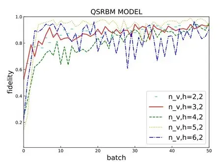
The fidelity of the QSRBM in figure 2(b) is slightly higher than that of the classical model when training the MNIST dataset.In order to save the computing power,we set the number of the hidden units to very small.As shown in figure 4,when the visible units are 5 and the hidden layer units are 2,the fidelity obtained by training is the highest.When the visible units are fixed,the hidden units determine the degree of the constraint of each training data on the model parameters.In the case of weight sharing,appropriately increasing the number of the hidden units may make the model learn better.On the other side,too many hidden units can lead to severe overfitting.Practically,the number of hidden units should be determined according to the actual situation.Therefore,one may infer that if the ratio of hidden units to visible units is slightly increased,the fidelity in our model on the training digital set may be probably higher.

Figure 4.The change of fidelity with the configuration number of visible units and hidden units when training Bernoulli distribution sets with QSRBM.
From figures 2–4,one can see that the training curve in the quantum model is not as smooth as that in the classical model.This is because the entire training data is used to train the parameters only once.Each time when a batch is performed,the new data is trained and the fidelity may increase or decrease,but the gradient descent algorithm ensures that the trend of training results is gradual convergence.
4.Summary and discussion
In summary,we have studied training digital image sets with variable QBMs.Numerical simulations showed that the QSRBM works well,while the QBM model does not.There is still some room for improvement in our model compared with other wellperformed classifiers [41],such as increasing the number of hidden units to improve the recognition rate.Despite such few resource conditions,the results of QSRBM are still close to the classical model in training data and fulfilling tasks.This illustrates that machine learning with quantum algorithms is feasible and promising.Particularly,the training results of QSRBM are better than that of QBM with fewer computing results,which definitely means that the proper algorithm is important in quantum machine learning.
Acknowledgments
This work was supported by the National Natural Science Foundation of China under Grant No.11725524,and the Hubei Provincal Natural Science Foundation of China under Grant No.2019CFA003.
杂志排行
Communications in Theoretical Physics的其它文章
- Preface
- Phase behaviors of ionic liquids attributed to the dual ionic and organic nature
- Chaotic shadows of black holes: a short review
- QCD at finite temperature and density within the fRG approach: an overview
- The Gamow shell model with realistic interactions: a theoretical framework for ab initio nuclear structure at drip-lines
- Effects of the tensor force on low-energy heavy-ion fusion reactions: a mini review
