QCD at finite temperature and density within the fRG approach: an overview
2022-10-22WeijieFu
Wei-jie Fu
School of Physics,Dalian University of Technology,Dalian,116024,China
Abstract In this paper,we present an overview on recent progress in studies of QCD at finite temperature and densities within the functional renormalization group (fRG) approach.The fRG is a nonperturbative continuum field approach,in which quantum,thermal and density fluctuations are integrated successively with the evolution of the renormalization group(RG)scale.The fRG results for the QCD phase structure and the location of the critical end point(CEP),the QCD equation of state(EoS),the magnetic EoS,baryon number fluctuations confronted with recent experimental measurements,various critical exponents,spectral functions in the critical region,the dynamical critical exponent,etc,are presented.Recent estimates of the location of the CEP from first-principle QCD calculations within fRG and Dyson–Schwinger equations,which pass through lattice benchmark tests at small baryon chemical potentials,converge in a rather small region at baryon chemical potentials of about 600 MeV.A region of inhomogeneous instability indicated by a negative wave function renormalization is found with μB ≿420 MeV.It is found that the non-monotonic dependence of the kurtosis of the net-proton number distributions on the beam collision energy observed in experiments could arise from the increasingly sharp crossover in the regime of low collision energy.
Keywords: QCD phase transition,chiral phase transition,QCD phase diagram,functional renormalization group
1.Introduction
One of the most challenging questions in heavy-ion physics arises from the attempt to understand how the deconfined quarks and gluons,i.e.the quark-gluon plasma(QGP),evolve into the confined hadrons.This evolution involves apparently two different phase transitions: one is the confinementdeconfinement phase transition and the other is the chiral phase transition related to the breaking and restoration of the chiral symmetry of QCD.When the strange quark is in its physical mass and the u and d quarks are massless,i.e.in the chiral limit,the chiral phase transition in the regime of small chemical potential in the QCD phase diagram,see e.g.figure 9,might be of second order,and belongs to the O(4)symmetry universality class [1,2].With the increase of the baryon chemical potential,the second-order phase transition might be changed into a first-order one at the tricritical point.When the u and d quarks are in their small,but nonvanishing physical masses,due to the explicit breaking of the chiral symmetry,the O(4)second-order chiral phase transition turns into a continuous crossover[3],which is also consistent with experimental measurements,see e.g.[4].The tricritical point in the phase diagram evolves into a critical end point (CEP),which is the end point of the first-order phase transition line at high baryon chemical potential or densities.
Although the phase transition at the CEP is of second order and belongs to the Z(2)symmetry universality class,the location of CEP and the size of the critical region around the CEP are non-universal.From the paradigm of the QCD phase diagram described above,one can easily find that the CEP plays a pivotal role in understanding the whole QCD phase structure in terms of the temperature and the baryon chemical potential.As a consequence,it becomes a very important task to search for and pin down the location of the CEP in the QCD phase diagram.Lattice simulations provide us with a wealth of knowledge of QCD phase transitions at vanishing and small baryon chemical potential,see e.g.[5–16],but due to the sign problem at finite chemical potentials,lattice calculations are usually restricted in the region of μB/T ≾2–3,where no signal of CEP is observed[17].Notably,recent estimates of the location of CEP from firstprinciple functional approaches,such as the functional renormalization group(fRG)and Dyson–Schwinger equations(DSE),which pass through lattice benchmark tests at small baryon chemical potentials,converge in a rather small region at baryon chemical potentials of about 600 MeV[18–20],and see also,e.g.[21]for related discussions.
Search for the CEP is currently underway or planned at many facilities,see,e.g.[4,22–33].Since the CEP is of second order,the correlation length increases significantly in the critical region in the vicinity of a CEP.Moreover,it is well known that fluctuation observables,e.g.the fluctuations of conserved charges,are very sensitive to the critical dynamics,and the increased correlation length would result in the increase of the fluctuations as well.Therefore,it has been proposed that a non-monotonic dependence of the conserved charge fluctuations on the beam collision energy can be used to search for the CEP in experimental measurements[34–36],see also [22].In the first phase of the Beam Energy Scan(BES-I)program at the relativistic heavy ion collider (RHIC)in the last decade,cumulants of net-proton,net-charge and net-kaon multiplicity distributions of different orders,and their correlations have been measured [37–44].Notably,recently a non-monotonic dependence of the kurtosis of the net-proton multiplicity distribution on the collision energy is observed with 3.1 σ significance for central gold-on-gold(Au+Au) collisions [42].
In this work,we would like to present an overview on recent progress in studies of QCD at finite temperature and densities within the fRG approach.The fRG is a nonperturbative continuum field approach,in which quantum,thermal and density fluctuations are integrated successively with the evolution of the renormalization group (RG) scale[45],see also [46,47].For QCD-related reviews,see,e.g.[48–55].Remarkably,recent years have seen significant progress in first-principle fRG calculations,for example,the state-of-the-art quantitative fRG results for Yang–Mills theory in the vacuum [56]and at finite temperature [57],vacuum QCD results in the quenched approximation[58],unquenched QCD in the vacuum [59–61]and at finite temperature and densities [18,62].
In this paper,we try to present a self-contained overview,which includes some fundamental derivations.Although new researchers in this field,e.g.students,may find these derivations useful,familiar readers could just skip over them.Furthermore,in this paper we focus on studies of fRG at finite temperature and densities,so we have to give up some topics,which in fact are very important for the developments and applications of the fRG approach,such as the quantitative fRG calculations to QCD in the vacuum [56,58,61].
This paper is organized as follows:in section 2 we introduce the formalism of the fRG approach,including the Wetterich equation,the flow equations of correlation functions,the technique of dynamical hadronization,etc.Moreover,we also give a brief discussion about Wilson’s recursion formula and the Polchinski equation,which are closely related to the fRG approach.In section 3 we discuss the application of fRG in the low energy effective field theories (LEFTs),including the Nambu–Jona-Lasinio (NJL) model and the quark-meson model.The relevant results in LEFTs,e.g.the phase structure,the equation of state(EoS),baryon number fluctuations,and critical exponents,are presented.In section 4 we turn to the application of fRG to QCD at finite temperature and densities.After a discussion about the flows of the propagators,strong couplings,four-quark couplings and the Yukawa couplings,we present and discuss the relevant results,e.g.the natural emergence of LEFTs from QCD,several different chiral condensates,QCD phase diagram and QCD phase structure,the inhomogeneous instability at large baryon chemical potentials,the magnetic EoS,etc.In section 5 we discuss the realtime fRG.After the derivation of the fRG flows on the Schwinger–Keldysh closed time path,one formulates the realtime effective action in terms of the ‘classical’ and ‘quantum’fields in the physical representation.The spectral functions and the dynamical critical exponent of the O(N) scalar theory are discussed.In section 6 a summary with conclusions is given.Moreover,an example for the flow equations of the gluon and ghost self-energies in Yang–Mills theory at finite temperature is given in appendix A.The Fierz-complete basis of four-quark interactions of Nf=2 flavors is listed in appendix B,and some useful flow functions are collected in appendix C.
2.Formalism of the fRG approach
We begin the section with a derivation of the Wetterich equation,i.e.the flow equation of the effective action,which is followed by a brief introduction about Wilson’s recursion formula and the Polchinski equation,since they are closely related to the fRG approach.Then,the fRG approach is applied to QCD.A simple method to obtain the flow equations of correlation functions,i.e.equation (61),is presented.An example for the flow equations of the gluon and ghost self-energies in Yang–Mills theory at finite temperature is given in appendix A.Finally,the technique of dynamical hadronization is discussed in section 2.5.
2.1.Flow equation of the effective action
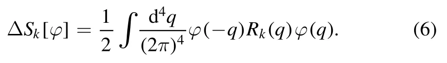
We begin with a generating functional for a classical actionS[]with an infrared (IR) regulator as follows
withRkab=Rkbafor bosonic indices andRkab=-Rkbafor fermionic ones.See e.g.[49]for discussions about generic regulators.We will see in the following that the IR cutoff k here is essentially the RG scale.
We proceed to taking a single scalar field φ for example,and the relevant regulator reads
It is more convenient to work in the momentum space.Employing the Fourier transformation as follows
one is led to
Here,the regulator has the following asymptotic properties which read

with a fixed q.In order to fulfill the aforementioned Requirement,viz.,only suppressing quantum fluctuations of momenta q ≾k selectively,one could make the choice as follows

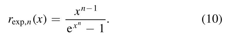
One may have already noticed that there are infinite regulators fulfilling equation (8).Here,we present two classes of regulators that are frequently used in the literature: one is the exponential-like regulator as follows

with
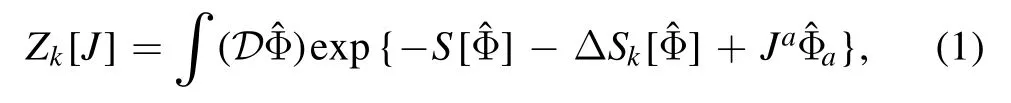
The sharpness of the regulator in the vicinity of q=k is determined by the parameter n,as shown in figure 1,where the exponential regulators with n=1 and 2 are depicted as functions of q with a fixed k.In figure 1 we also plot another commonly used regulator,i.e.the flat or optimized one[63,64],which reads
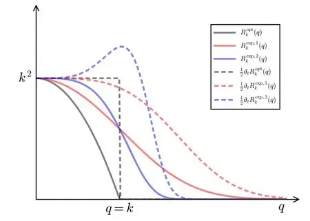
Figure 1.Comparison of several different regulators and their derivatives with respect to the RG scale k as functions of the momentum q with a fixed k.

with
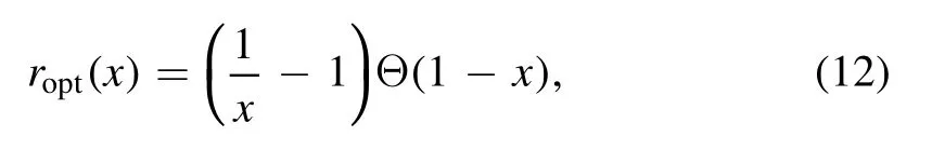
where Θ(x) is the Heaviside step function.Moreover,the derivative of the regulator with respect to the RG scale k,to wit,

is also shown in figure 1,where t is usually called as the RG time.For more discussions about regulators,see,e.g.[65].

It is more convenient to use the generating functional for connected correlation functions,viz.,which is also known as the Schwinger function.Then,the expected value of a field is readily obtained as
and the propagator reads
where the subscript c stands for ‘connected’.Moreover,Legendre transformation to the Schwinger function leaves us immediately with the one-particle irreducible (1PI) effective action,which reads

In order to take both bosonic and fermionic fields into account altogether,we adopt the notation introduced in [49],to wit,

with
Inserting equation(18)into(17)and differentiating both sides of equation (17) with respect to Φa,one is led to
where by,the propagator in equation(16)is readily written as the inverse of the second-order derivative of Γk[Φ]w.r.t.Φ,i.e.

with
We proceed to consider the evolution of the Schwinger function with the RG scale,i.e.the flow equation of Wk[J],which is straightforwardly obtained from equations (1) and(14).The resulting flow reads
where we have introduced a notation super trace for compactness,which can also be expressed as
The factor γ in the equation above indicates that the super trace provides an additional minus sign for fermionic degrees of freedom.Note that in deriving equation(23)we have used the relation in equation (16).Applying Legendre transformation in equation (17) to the flow equation of Schwinger function in equation(23)once more,one immediately arrives at the flow equation of the effective action,as follows
which is the Wetterich equation [45].Note that the flow equation of effective action in equation (25) would be modified when the dynamical hadronization is encoded,see equation (80).In section 2.3 we would like to give an example for the application of fRG,and postpone discussions of the dynamical hadronization in section 2.5.
2.2.From Wilson’s RG to Polchinski equation
The idea encoded in the Wetterich equation in equation (25)is that integrating out high momentum modes leaves us with an RG rescaled theory,and this theory is invariant at a second-order phase transition.This idea is also reflected in Wilson’s RG and Polchinski equation,to be discussed in this subsection.
2.2.1.Wilson’s RG and recursion formula.Here we follow[66]and begin with the Ginzburg–Landau Hamiltonian K≡H[σ]/T,which reads
Then one separates the field into two parts as follows
with
where L denotes the size of the system,Λ is a UV cutoff scale and Λ-1can be regarded as the lattice spacing.The planewave expansion in equation(28)can also be replaced by that in terms of localized wave packets Wz(x),i.e.the Wannier functions for the band of plane waves Λ/2<q<Λ,that is,
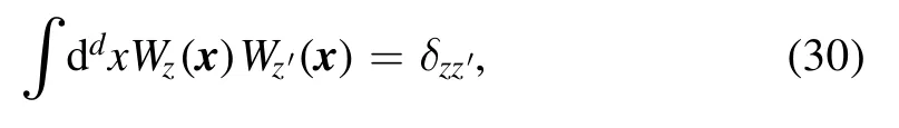
Obviously,the wave packets have the property Wz(x)~0,if∣x-z∣≫ 2Λ-1,and one also has
i.e.they are orthonormal.Substituting equation(27)into(26)and performing a functional integral overσ˜(x) or ˜σz,one arrives at
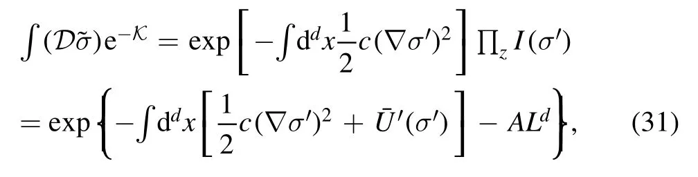
with
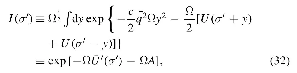
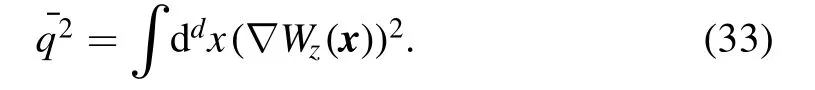
where Ω is the volume of a block or the wave packet;the constant A is determined by the condition(0)=0;the mean square wave vector of the packet reads
In deriving equation (31),one has neglected the overlap between wave packets,the variation ofσ′(x) and the absolute value of Wz(x) within a block,and see [66–68]for details.Note that equation (31) is just the first step of the Kadanoff transformation.
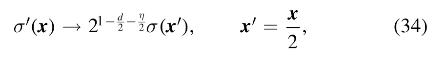
The second step of the Kadanoff transformation is to make a replacement for the remaining fieldσ′ and the coordinate in equation (31) as follows
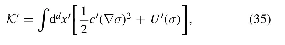
and thus one is left with
with
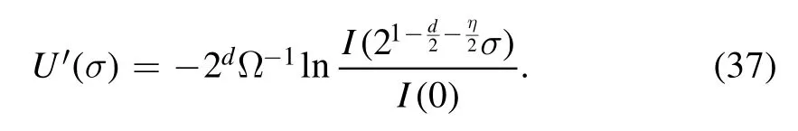
and
In order to makec′=csatisfied,one adopts η=0.Choosing an appropriate value of c,such that
and defining
one arrives at
with
which is Wilson’s recursion formula [67,68].Note that the constant prefactor Ω1/2in equation (32) is irrelevant.
2.2.2.Polchinski equation.In section 2.2.1 we have discussed the viewpoint of Wilson’s RG,that is,integrating out modes of high scales successively leaves us with a low energy theory that evolves with the RG scale.This idea is also applied to a generic quantum field theory within the formalism of the functional integral,due to Polchinski [69].We begin with a generating a functional for a scalar field theory in four Euclidean dimensions with a momentum cutoff,i.e.
with a cutoff function given by
Evidently,here Λ0plays a role as a UV cutoff scale,and Lintin equation (42) is the interaction Lagrangian at the scale Λ0,that for example reads
where we have used the notation in[69],andρ0a's stand for bare quantities.
One would like to integrate out the high momentum modes of φ and reduce the UV cutoff Λ0to a lower value,say Λ.Inthe meantime,onechooses∣m2∣<ΛandJ(p)=0for p2>Λ2.Aswe have discussed insection 2.2.1,when high momentum modes are integrated out,new effective interactions,included in the potentialU′ in equation (35) or the interaction Lagrangian Lintin equation(42),are generated.Thus,one is led to the following functional integral
If one wishes to take the generating functional Z[J,L,Λ]on the l.h.s.of the equation above to be independent of the scale Λ,i.e.
the following evolution equation for the interaction Lagrangian in equation (45) has to be satisfied,to wit,
which is the Polchinski equation [69].
2.3.Application to QCD
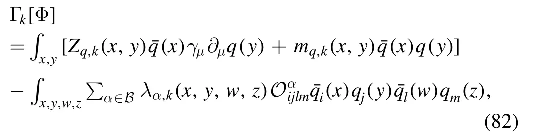
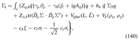
In this section,we would like to apply the formalism of fRG discussed above to an effective action of rebosonized QCD in[18].The truncation for the Euclidean effective action reads
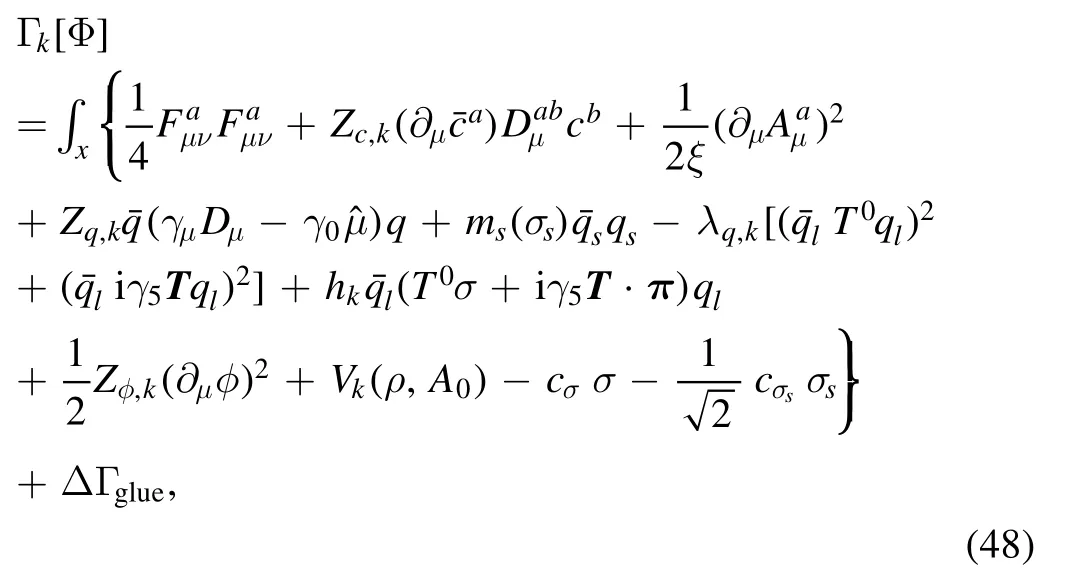
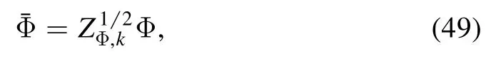
The first line on the r.h.s.of equation (48) denotes the classical action for the glue sector,while its non-classical contributions are collected in ΔΓglue.The gauge parameter ξ=0,i.e.the Landau gauge,is commonly adopted in the computation of functional approaches.The wave function renormalization ZΦ,kof field Φ is defined as
with the renormalized field.The gluonic field strength tensor reads

Note that although different strong couplings are identical in the perturbative region,they can deviate from each other in the nonperturbative or even semiperturbative regime [56–58,61],and see also relevant discussions in section 4.2.Therefore,it is necessary to distinguish different strong couplings.The renormalized strong couplings in the glue sector read
whereλA3,k,λA4,kandstand for the three-gluon,fourgluon,ghost-gluon dressing functions,respectively,as shown in equations(A42),(A48),(A36).In equation(50)the gluonic strong couplings are denoted collectively as.In the same way,the quark-gluon coupling reads
with the quark-gluon dressing function.The covariant derivative in the fundamental and adjoint representations of the color SU(Nc) group reads
respectively.Here fabcis the antisymmetric structure constant of the SU(Nc) group,determined from its Lie algebra [ta,tb]=ifabctc,where the generators have the normalization Trta tb=(1 、2)δab.
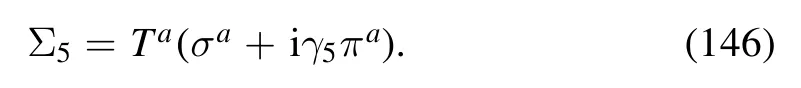
In equation (48) the formalism of Nf=3 flavor quark is built upon that of Nf=2 by means of the addition of a dynamical strange quark qs,whose constituent quark mass ms(σs) is determined self-consistently from an extended effective potential of SU(Nf=2),and see [18]for more details.Therefore,we have the quark field q=(ql,qs),where the u and d light quarks are denoted by ql=(qu,qd).The light quarks interact with themself through the four-quark coupling in the σ–π channel,and they are also coupled with the σ and π mesons via the Yukawa coupling.Here Ti(i=1,2,3)are the generators of the group SU(Nf=2) in the flavor space with TrTi Tj=(1 2)δijandT0=with Nf=2.In equation (48)=diag (μu,μd,μs)stands for the matrix of quark chemical potentials.
The effective potential in equation (48) can be decomposed into two parts as follows

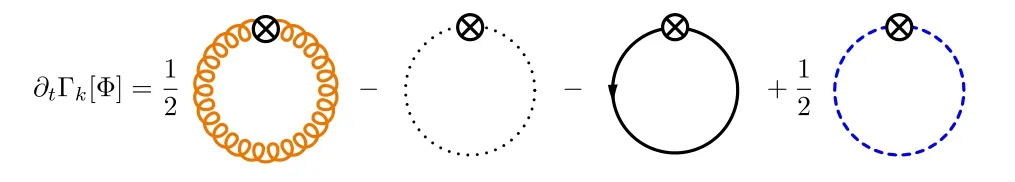
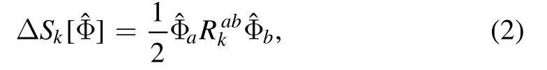
Figure 2.Diagrammatic representation of the flow equation for QCD effective action.The lines denote full propagators for the gluon,ghost,quark,and meson,respectively.The crossed circles stand for the infrared regulators.
The first term on the r.h.s.of the equation above is the glue potential,or the Polyakov loop potential.The temporal gluon field A0is intimately related to the Polyakov loop L[A0],see e.g.[70];the second term is the mesonic effective potential of Nf=2 flavors,which is O(4)-invariant with ρ=φ2/2.Moreover,in the effective action in equation (48) cσandσcsare the parameters of explicit chiral symmetry breaking for the light and strange scalars σ,σs,respectively.
Applying the fRG flow equation in equation (25) to the QCD effective action in equation (48),one immediately arrives at the QCD flow equation,which is depicted in figure 2.One can see that the flow of effective potential receives contributions from the gluon,ghost,quark,and composite fields separately,each of which is a one-loop structure.It should be emphasized that,although it is a oneloop structure,the flow is composed of full propagators which are in turn dependent on the second derivative of the effective action,see equation(21).Thus,the flow equation in figure 2 a functional self-consistent differential equation,which will be explored further in the following.
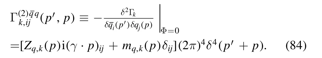
2.4.Flow equations of correlation functions
Combining equation (21) one can reformulate Wetterich equation in equation (25) slightly such that
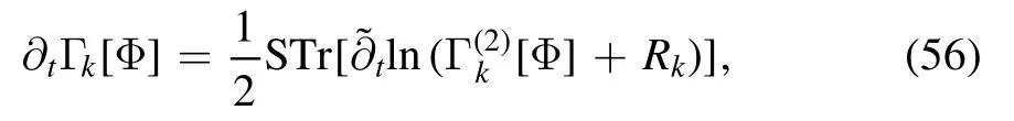
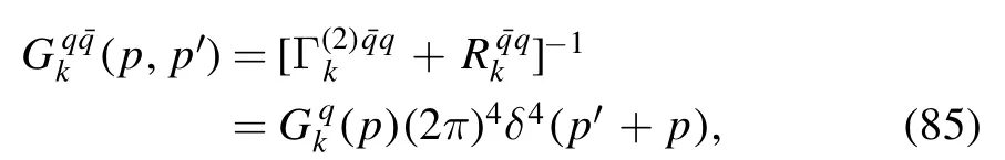
where the differential operator with a tilde,,hits the RGscale dependence only through the regulator.Note that Γ(k2)[Φ]in equation (56) is a bit different from that in equation (22),and here the factorγabis absorbed inΓ(k2)[Φ].A convenient way to take this into account is to use the definition as follows
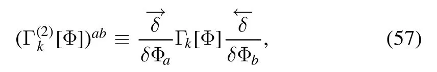
where the left and right derivatives have been adopted.
In order to derive the flow equations for various correlation functions of different orders,it is useful to express Γ(k2)in equation(57)in terms of a matrix,and the indices of matrix correspond to different fields involved in the theory concerned,e.g.Φ=(A,c,,q,,σ,π)in section 2.3.This matrix is also called as the fluctuation matrix[71].Then,one can make the division as follows
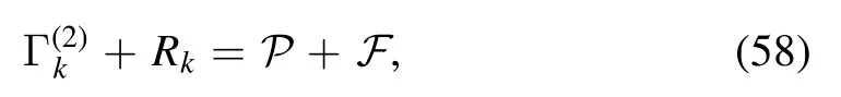
where P is the matrix of two-point correlation functions including the regulators,and its inverse gives rise to propagators;F is the matrix of interaction which includes n-point correlation functions with n >2,and thus terms inF have the field dependence.Substituting equation (58) into (56) and making the Taylor expansion in order ofF P,one arrives at
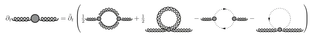
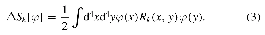
Figure 3.Diagrammatic representation of the flow equation for the gluon self-energy in Yang–Mills theory,where the last diagram arises from the non-classical two-ghost–two-gluon vertex.
from which it is straightforward to obtain the flow equations for various inverse propagators and vertices at some appropriate orders.
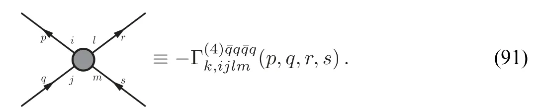
Moreover,one can also employ some well-developed Mathematica packages,e.g.DoFun [72,73],QMeS-Derivation [74],to derive the flow equations for correlation functions.We refrain from elaborating on details about the usage of these Mathematica packages in this review,which interested readers can find in the references above,but rather would like to introduce another easy-to-use approach to derive the flow equations described in detail in section 2.4.1.
2.4.1.A simple approach to derivation of flow equations of correlation functions.We proceed with defining a generic 1PI n-point correlation function or vertex,as follows
where 〈Φ〉 denotes the value of Φ on its equation of motion(EoM).The flow equation of vertexVk(n)in equation(60)can be represented schematically as the equation as follows
Note that the one-loop diagrams on the r.h.s.are comprised of full propagators and vertices.As we have mentioned above,the partial derivative with a tildehits the RG-scale dependence only through the regulator,and thus its implementation on diagrams would give rise to the insertion of a regulator for each inner propagator.
As an example,we present the flow equation of the gluon self-energy in Yang–Mills theory in figure 3.One can see that it receives contributions from the gluon loop,the tadpole of the gluon,the ghost loop,and the tadpole of the ghost.Note that the last diagram on the r.h.s.of the equation in figure 3 arises from the non-classical two-ghost–two-gluon vertex.Remarkably,the factors in front of each diagram are in agreement with those in the perturbation theory.It,however,should be emphasized once more that although these diagrams are very similar with the formalism of perturbation theory,they are essentially nonperturbative,since both propagators and vertices in these diagrams are the full ones.
In order to let readers be familiar with the computation in fRG,we present some details about the flow equations of the gluon and ghost self-energies in the Yang–Mills theory at finite temperature in appendix A.
2.5.Dynamical hadronization
In section 2.3 we have mentioned that the mesonic fields in equation (48) are not added by hands.On the contrary,these composite degrees of freedom are dynamically generated from fundamental ones with the evolution of the RG scale from the ultraviolet (UV) toward the infrared (IR) limit.This is done via a technique called dynamical hadronization,which was proposed in [71,75],and subsequently the formalism was further developed in [49].Notably,recently the explicit chiral symmetry breaking and its role within the dynamical hadronization have been investigated in detail in [18],and a flow of dynamical hadronization with manifest chiral symmetry is put forward therein.In this section,we follow [18]and present the derivation of flow equation of the dynamical hadronization.
We denote the original or fundamental degrees of freedom in QCD aswith the expected valueφ=〈〉,where as composite degrees of freedom are introduced via a RG scale k-dependent composite field[49,71,75],which is a function of the fundamental field.Then the superfield reads

with

The generating functional in equation (1) is modified a bit such that
where the external source J=(Jφ,Jφ) withJφ=is conjugated to the field Φ=(φ,φk),distinguished with different labels of indices,i.e.

The regulator of bilinear fields in equation (64) reads

The effective action is obtained via a Legendre transformation to the Schwinger function as shown in equation (17).Note that the term of explicit chiral symmetry breaking in the effective action,e.g.-cσσ or-in equation (48),does not contribute to the flow of effective action,and thus the effective action can always be decomposed into that in the case of chiral limit plus an explicit chiral symmetry breaking term.We follow [18]and separate the explicit breaking out,such that
where we have concentrated on the case of Nf=2,which can be easily extended to include the strange quark.in equation (67) stands for the effective action without the explicit chiral symmetry breaking.From equation (67),one arrives at
with

i.e.

Equation(68)combined with equation(17)leaves us with the relation for Schwinger functions as follows

where one has


It is straightforward to obtain
Inserting equation(75)into(74)and then to(73),one is led to
where equation (16) has been used.Employing
and
one arrives at
Given the relation in equation (68) and the fact that cσis independent of the RG scale k,we finally obtain the flow equation of effective action with dynamical hadronization,to wit,
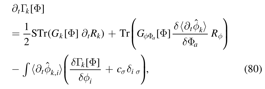
where some summations for the indices{a}and{i}as shown in equation (65) have been replaced with the super trace and trace,respectively;the integral over the spacetime coordinate is recovered for the last term on the r.h.s.of equation (80).The propagator Gk,iain equation(79)is relabeled withGk,φiΦathat has a clearer physical meaning.One can see that in comparison to equation (25),there are two additional terms,i.e.the last two on the r.h.s.of equation (80),in the flow equation of the effective action.These additional terms arise from the RG scale-dependent composite field in equation (63),and they can be employed to implement the Hubbard–Stratonovich transformation for every value of the RG scale,which eventually transfers the degrees of freedom from quarks to bound states.
3.Low energy effective field theories
Prior to discussing the properties of the QCD matter at finite temperature and densities in section 4,in this section,we would like to apply the formalism of fRG in section 2 to low energy effective field theories first.We adopt two commonly used formalisms of LEFTs,i.e.the purely fermionic NJL model in section 3.1 and the quark-meson (QM) model in section 3.2,respectively.
3.1.NJL model
One prominent feature characteristic of the nonperturbative QCD is the dynamical chiral symmetry breaking,which is regarded as being responsible for the origin of the~98%mass of visible matter in the Universe [76–79],in contradistinction to the~2% electroweak mass.Within the fRG approach,the dynamical breaking or restoration of the chiral symmetry is well encoded in the four-fermion flows,which is illustrated briefly in what follows.For more details,see,e.g.[80,81–89]and a related review [53].
Using the method to derive the flow equation for a generic vertex as shown in equation(61),one is able to obtain the flow equation of four-quark coupling,depicted schematically in figure 4.Here we refrain from going into the details of a realistic calculation,but rather try to infer behaviors of the four-quark flow connected to the breaking or restoration of the chiral symmetry.It follows from figure 4 that the β function for the dimensionless four-quark coupling≡kλ2 reads
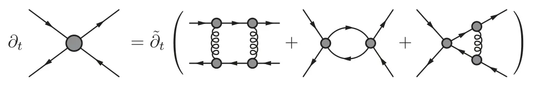
Figure 4.Schematic representation of the flow equation for the fourquark coupling.Those on the r.h.s.of equation stand for three classes of diagrams contributing to the flow of four-quark interaction,that is,the two-gluon exchange,purely self-interacting four-quark coupling,and mixture of the quark-gluon and four-quark interactions,respectively.Here,diagrams of different channels of momenta are not distinguished and prefactors for each diagram are not shown.

with the dimension of spacetime d=4 and the strong coupling g.Note that apart from the first term on the r.h.s.of equation(81)arising from the dimension of λ,the remaining three terms correspond to the three classes of diagrams in figure 5 one by one,and their coefficients are denoted by a,b,c,respectively.Further computation indicates one has a >0 and c >0 [90].
In the left panel of figure 5,a typical β function is plotted as a function of the dimensionless four-quark coupling schematically in different cases.When the gauge coupling g is vanishing and at zero temperature,there are two fixed points:one is the Gaussian IR fixed point=0,the other the UV attractive fixed point at a nonvanishing,and they are shown in the plot by red and purple dots,respectively.The position of the UV fixed point determines a critical value,which is necessitated in order to break the chiral symmetry,since only when>,the four-quark coupling grows large and eventually diverges with the decreasing RG scale.When the temperature is turned on,the IR fixed point remains at the origin while the UV fixed point move towards right,as shown by the red dashed line.As a consequence,the broken chiral symmetry in the vacuum is restored at a finite T,if one has a value ofwith(T=0)<<(T).When the strong coupling is nonzero,the parabola of β function moves downwards globally as shown by the blue curve in the left panel of figure 5.There is a critical value of the strong coupling,say gc,once one has g >gc,the whole curve of the beta function is below the line β=0,which implies that the chiral symmetry breaking is bound to occur,no matter how large the initial value ofis.
The four-fermion flow is also well suited for an analysis of the chiral symmetry breaking in an external magnetic field.The inclusion of a magnetic field would modify the four-quark flows as well as the fixed-point structure[80,83].The plot in the right panel of figure 5 is obtained in[80],which demonstrates that in the case of a magnetic field the flow pattern of the four-quark coupling has been changed and the chiral symmetry is always broken.This is in fact due to the dimensional reduction under a finite external magnetic field.Moreover,it is found that once the in-medium effects of temperature and densities are implemented,long-range correlations are screened and the vanishing critical coupling shown by the red line in the right panel of figure 5 is not zero anymore [80].
Recently,a Fierz-complete four-fermion model is employed to investigate the phase structure at finite temperature and quark chemical potential,and it is found that the inclusion of four-quark channels other than the conventionally used scalar-pseudoscalar ones not only plays an important role in the phase diagram at large chemical potential,but also affects the dynamics at small chemical potential[85].The related fixed-point structure is analyzed at the finite chemical potential in the Fierz-complete NJL model,and it is found the dynamics are dominated by diquarks at large chemical potential [86].Resorting to the fRG flows of four-quark interactions,one is able to observe the natural emergence of the NJL model at intermediate and low energy scales from fundamental quark-gluon interactions [87].EoS of nuclear matter at supranuclear densities is also studied in the Fierz-complete setting [88],and a maximal speed of sound is found at supranuclear densities,which is related to the emergence of color superconductivity in the regime of high densities,i.e.the formation of a diquark gap,see also[89]for details.Moreover,the UA(1)symmetry and its effect on the chiral phase transition are investigated in the Fierzcomplete basis [91].
Up to now,we have only discussed the chiral symmetry and its breaking by means of the four-fermion flows.As mentioned in the beginning of section 3.1,a direct consequence of the dynamical chiral symmetry breaking is the production of mass,which is our central concern in the following.Here,we discuss recent progress in understanding the quark mass generation and the emergence of bound states in terms of RG flows [92].Considering only the quark degrees of freedom in equation (48) and extending the scalar-pseudoscalar four-quark interaction to a Fierz-complete set of Nf=2 flavors,denoted byB in the following,one arrives at a RG-scale dependent effective action,given by
with Φ=(q,)and ∫x,…≡∫d4x∫….Herestands for the four-quark operator of channel α,where the indices i,j,l,m run over the Dirac,flavor and color(Nc=3)spaces,and the related coupling strength is given by λα,k.In the same way,the summation is assumed for repeated indices.In appendix B ten independent Fierz-complete channels of four-quark interactions of Nf=2 flavors are presented.
The two-quark correlation function reads
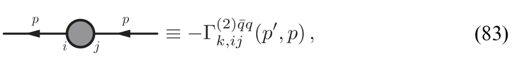
with
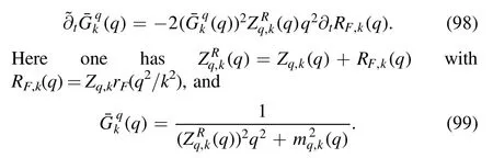
Then one arrives at the quark propagator with an IR regulator,viz.,
with a fermionic regulator given by

and
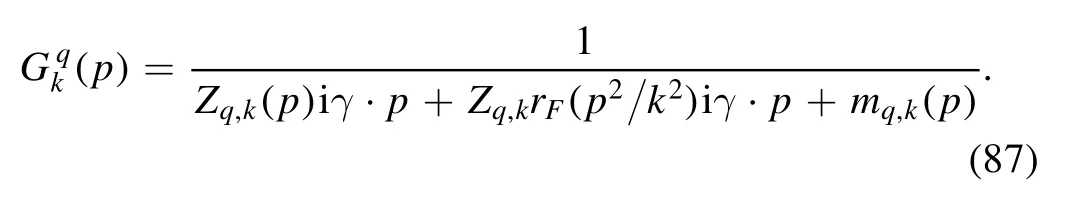
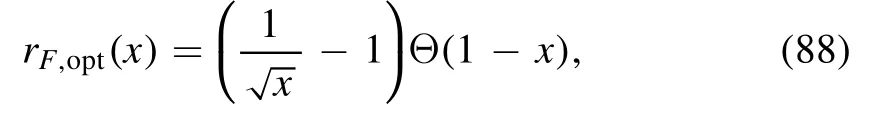
Note that the fermionic regulator in equation (86),in comparison to the bosonic one in equations (9) and (11),is implemented in the vector channel rather than the scalar one,which guarantees that the chiral symmetry is not broken by the regulator.In the same way,one is allowed to make a choice for the specific formalism of the fermionic regulator,e.g.the optimized one,
or the exponential one in equation (10),
and even the simplest exponential regulator as follows
The four-quark correlation function reads
with
where the symmetric and antisymmetric four-quark couplings read
Neglecting the diagrams including the quark-gluon interaction in figure 4 and showing explicitly different channels of momenta,one is able to obtain the flow equation of four-quark coupling within the purely fermionic effective action in equation (82),shown diagrammatically in the second line of figure 6.We also depict the flow equation of the two-quark correlation function,i.e.the quark self-energy,in figure 6.
3.1.1.Quark mass production.Following [92]we assume that the antisymmetric four-quark couplingsλαA,k's in equation (94) are vanishing in order to simplify calculations.Then,equations (93) and (94) leave us with

and its flow equation reads
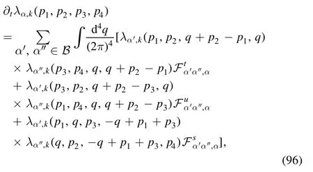
where the superscripts t,u,and s of coefficientF's indicate that the relevant terms in equation (96) arise from the corresponding loop diagrams in the flow of four-quark coupling in figure 6.The coefficientF's depend on the quark propagators and regulators and see [92]for their explicit expressions.The flow of quark mass is readily obtained by projecting the flow equation of the quark selfenergy in the first line in figure 6 onto the scalar channel,which reads
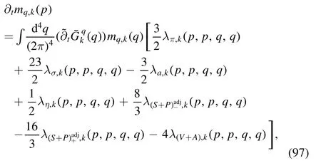
with
For the moment,we assume Zq,k=1 and use the truncation as follows
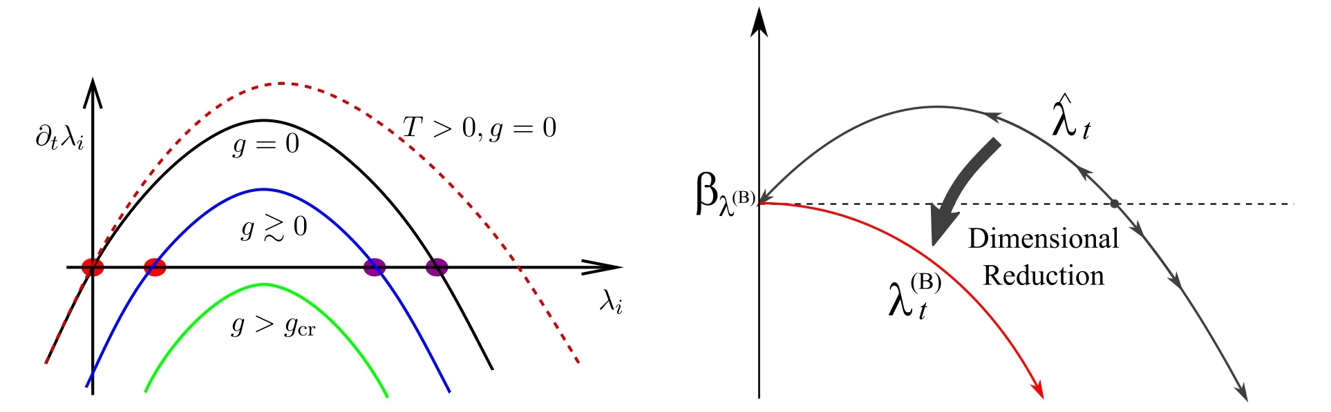
Figure 5.Left panel:Sketch of a typical β function for the dimensionless four-quark coupling≡kλ2 in different cases,where g is the gauge coupling and T is the temperature.The plot is adapted from[90].Right panel:Comparison between the β functions of with and without an external magnetic field.The inclusion of a magnetic field results in that the chiral symmetry is always broken due to dimensional reduction.The plot is adapted from [80].
that is,neglecting the momentum dependence of the fourquark coupling and quark mass.The dimensionless fourquark coupling=λα,kk2and quark mass=mq,k、kare also very useful in the following.
In order to focus on the mechanism of quark mass production,we make a further approximation as follows
i.e.only keeping the scalar-pseudoscalar σ and π channel.Then the flow equations in equations (96) and (97) are simplified as
and
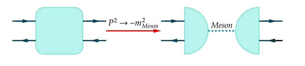
Figure 7.Schematic diagram showing the emergence of resonance at the pole of relevant meson mass from the four-quark vertex,where the square and half-circles stand for the full four-quark and quarkmeson vertices,respectively.The dashed line denotes the meson propagator.
respectively.Here we have used the dimensionless variables,which entails that the RG scale k-dependence for these equations is removed.Numerical results of the RG flows ofandin equations (104) and (105) can be found in [92].
3.1.2.Natural emergence of bound states.Properties of bound states of quarks or antiquarks,e.g.the pions and nucleons,in principle can be inferred from the relevant fourpoint and six-point vertices of quarks,in some specific channels and regimes of momenta [93].In figure 7 a sketch map shows how this happens in the example of mesons.The square denotes a four-point vertex of quark and antiquark.If the total momentum of a quark and an antiquark,denoted by P here,is in the Minkowski spacetime and in the vicinity of the on-shell pole mass of a meson in some channel,i.e.P2~-mm2eson,the full four-quark vertex can be well described by a resonance of the meson,as shown on the r.h.s.of figure 7,where two quark-meson vertices are connected with the propagator of meson.Therefore,one has to calculate the full four-quark vertex or quark-meson vertex in some specific regime of momentum,which is usually realized by resuming a four-quark kernel to the order of infinity in the formalism of Bethe–Salpeter equations[94,95].Note that the necessary resummation for the four-quark vertex is well included in the flow equation of four-quark couplings in equation(96),and it is,therefore,natural to expect that the RG flows are also well-suited for the description of bound states as the same as the quark mass production in section 3.1.1.Moreover,the advantage of RG flows is evident,that is,the self-consistency between the bound states encoded in the flow of four-quark vertices in equation (96)and that of quark mass gap in equation (97) can be well guaranteed,once a truncation is made on the level of the effective action,such as that in equation (82).
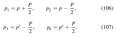
In order to investigate the resonance behavior of fourquark vertices in equation (96),one has to go beyond the truncation in equation (100)and include appropriate momentum dependence for the four-quark vertices.The external momenta of couplings in equation (96) are parameterized as follows
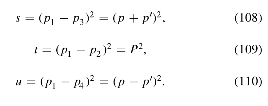
Then,one is left with the relevant Mandelstam variables given by
In the following,we focus on the π meson and assume,that the total momentum of quark and antiquark in the tchannel is near the regime of on-shell pion mass,viz.,one has the t-variableP2~-mπ2in equation (109).Consequently,the four-quark coupling of the pion channel would be significantly larger than those of other channels,and its dependence on external momenta would be dominated by the t-variable.Thus,one is allowed to make the approximation as follows
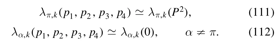
Furthermore,insofar as the four-quark vertices on the r.h.s.of the flow of coupling in the second line of figure 6,a simple analysis of relevant momenta for each vertex indicates,that the t-variable dependence is only required to be kept for the vertices in the diagram of t channel,i.e.the first diagram.One is thus allowed to simplify the flow equation of λπ,kin equation (96) as

with two coefficients given by

and
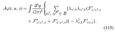
Note that all the four-quark couplings in equation (115) are momentum-independent.If one adopts furtherp=p′=0 in equations (106) and (107),two Mandelstam variables are vanishing,i.e.s=u=0,and one arrives at
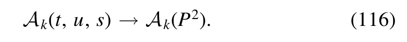
One is able to observe the natural emergence of a bound state arising from the resummation of the four-quark vertex from equation (113),whose solution is readily obtained once the last term on the r.h.s.is ignored.One has
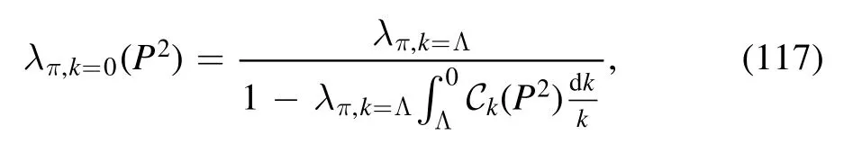
with λπ,k=Λthe four-quark coupling strength of the pion channel at the UV cutoff,which is independent of external momenta.Evidently,when a value of P2is chosen appropriately,such that the denominator in equation (117)is vanishing,the four-quark coupling in the IR λπ,k=0is divergent.As a consequence,one can employ this condition to determine the pole mass of the bound state,i.e.the pion mass,which reads
When the coefficientAk(P2)in equation (113) is taken into account,there is no analytic solution anymore.However,as shown in [92],the direct numerical calculation of equation (113) indicates that the qualitative behavior of the pole displayed by equation (115) is not changed,and more related numerical results of bound states are presented in[92].
3.2.Quark-meson model
In this section,we discuss another formalism of the low energy effective field theories,i.e.the quark-meson model,which in principle can be obtained from the NJL model via the bosonization with the Hubbard–Stratonovich transformation.The effective interactions between quarks and mesons in the rebosonized QCD effective action in equation (48),and their natural emergence resulting from the RG evolution of fundamental degrees of freedom will be discussed in detail in section 4.4.There is a wealth of studies in the literature relevant to the QM model within the fRG approach,see,e.g.[50,96–151].
For the moment,we only consider the degrees of freedom of quarks and mesons and their interactions via the Yukawa coupling in equation (48).The Nf=2 flavor QM effective action reads
Note that explanations for most notations in equation (119)can be found in section 2.3 below equation(48).The effective potential in equation (119) can be decomposed into a sum of the contribution from the glue sector and that from the matter sector,which corresponds to the first and last two loops of the flow in figure 2,respectively.Thus,one is led to

where the first term on the r.h.s.is the glue potential or the Polyakov loop potential,since it is usually reformulated by means of the Polyakov loop L(A0),and the latter can be calculated through the flow equation within the QM model.In the following,we still use Vk(ρ) to stand for Vmat,kfor simplicity in a slight abuse of notation.
3.2.1.Flow of the effective potential.The flow equation of the effective potential reads
with the threshold functions given by
and
where the bosonic distribution function reads
and the fermionic one
The quark and meson anomalous dimensions in equation (121) are given by
computation of which can be found in section 4.1.
There are two classes of methods to solve the flow equation of the effective potential in equation (121).The methods of the first class capture local properties of the potential and are very convenient for numerical calculations,but fail to obtain global properties of the potential.A typical method in this class is the Taylor expansion of the effective potential.On the contrary,the methods in the other class are able to provide us with the global properties of the potential,but usually,their numerical implements are relatively more difficult.The second class includes the discretization of the potential on a grid [97],the pseudo-spectral methods[152–155],e.g.the Chebyshev expansion of the potential[151],the discontinuous Galerkin method [156,157],etc.In what follows we give a brief discussion about the Taylor expansion and the Chebyshev expansion of the potential.
The Taylor expansion of the effective potential reads
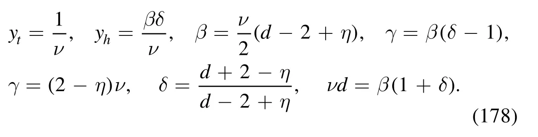
with the expansion coefficients λn,kand the expansion point кkthat might be k-dependent,where Nvis the maximal expanding order in the calculations.Reformulating equation (129) in terms of the renormalized variables,one is led to
with
Substituting equation (130) into the left hand side of equation (121),one arrives at
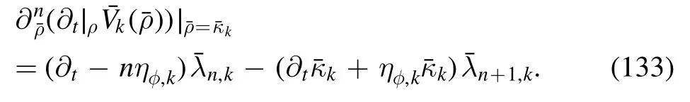
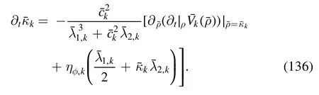
If the expansion point кkis independent of k,i.e.∂tкk=0,which is usually called the fixed point expansion,the expression in the second bracket on the r.h.s.of equation(133)is vanishing.One can see that in this case,the expansion coefficients of different orders in equation (130) decouple from each other in the flow equations,which results in an improved convergence for the Taylor expansion and better numerical stability [116].Another commonly used choice is the running expansion,where of one expands the potential around the field on the EoS for every value of k,that is,
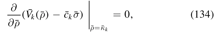
with
Here c is independent of k.Then one arrives at the flow of the expansion point,as follows
For more discussions about the fixed and running expansions,see,e.g.[59,116,118,128,148,158].In the same way,the field dependence of the Yukawa coupling,i.e.hk(ρ) can also be studied within a similar Taylor expansion [116,148],which encodes higher-order quark-meson interactions.Moreover,the effects of the thermal splitting for the mesonic wave function renormalization in the heat bath are also investigated in [148].
As for the Chebyshev expansion,the effective potential reads
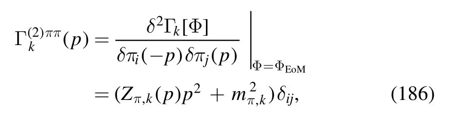
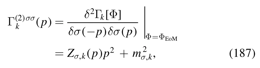
with the Chebyshev polynomialsTn()and the respective expansion coefficients cn,k.Then,one arrives at the flow of the effective potential as follows
where the field dependence of the meson wave function renormalization Zφ,k(ρ) as well as the meson anomalous dimensionηφ,k()is taken into account.Note that the coefficients dn,kare related to cn,kthrough a recursion relation as shown in [151].The flow equations of the coefficients in equation (137) are given by
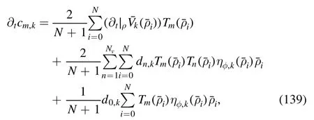
where the summation for i is performed on N+1 zeros of the polynomialTN+1().
3.2.2.Quark-meson model of Nf=2+1 flavors.The effective action for the Nf=2+1 flavor QM model,see,e.g.[109,110,128,140,143,147],reads
where the scalar and pseudoscalar mesonic fields of nonets are in the adjoint representation of the U(Nf=3) group,i.e.


where [,Σ]denotes the commutator between the matrix of chemical potentials and the meson matrix in equation (141).Note that although mesons do not carry the baryon chemical potential,they might have chemical potentials for the electric charge and the strangeness.The quark chemical potentials are related to those of conserved charges through the relations as follows
For the Yukawa coupling,one has
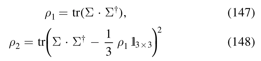
In contradistinction to the two-flavor case,the effective potential in equation (140) is a function of two chiral invariants,to wit,
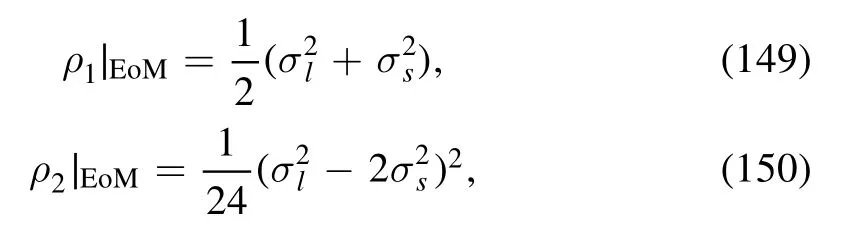
which are both invariant not only under SUA(3) but also UA(1).On the EoM these two invariants read
where the light and strange fields are related to the zeroth and eighth components in equation(141)through the relationship as follows
The term of Kobayashi–Maskawa-’t Hooft determinant in equation (140) preserves SUA(3) while breaking UA(1) with
and the breaking strength is described by the coefficient cA.The light and strange quark masses read
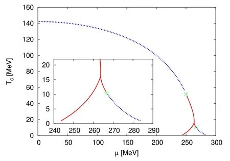
Figure 8.Phase diagram of the Nf=2 flavor QM model in the chiral limit in the plane of the temperature and quark chemical potential obtained with the discretization of the potential on a grid in[97].The plot is adapted from [97].
and the pion and kaon decay constants are given by
where σland σsare on their respective equations of motion.For more discussions about the flow equations in the Nf=2+1 flavor QM model,see the aforementioned references in this section.
3.2.3.Phase structure.In figure 8 the phase diagram of the Nf=2 flavor QM model in the chiral limit obtained in[97]is shown.In order to investigate the phase structure,especially in the regime of large chemical potential,the global information of the effective potential in equation (121) is indispensable.Thus,the potential is discretized on a grid to resolve the flow equation and see [97]for more details.One can see that in the region of small chemical potentials,there is a second-order chiral phase transition denoted by the blue dashed line.With the decrease of the temperature,the secondorder phase transition is changed into the first-order one at the tricritical point denoted by a green asterisk.The red solid lines stand for the first-order phase transition.Moreover,with the further decrease of the temperature,one observes that the first-order phase transition splits into two phase transition lines,one of which even evolves again into the second-order phase transition at high chemical potentials.Note that the first-order phase transition line backbends at high chemical potentials [135].
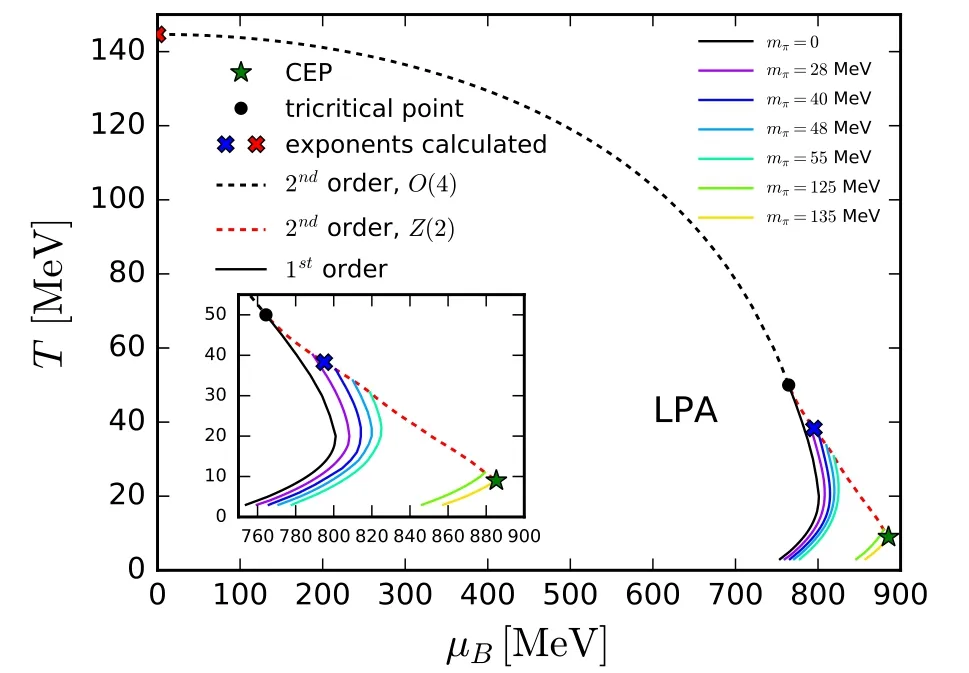
Figure 9.Phase diagram of the Nf=2 flavor QM model in the T–μB plane obtained with the Chebyshev expansion of the potential in[151].The plot is adapted from [151].
Figure 10.Phase diagram of the Nf=2 flavor QM model in the T–μq plane obtained with a discontinuous Galerkin method in [157],where the color stands for the value of the order parameter.The plot is adapted from [157].
In figure 9 the phase diagram of the Nf=2 flavor QM model obtained with the Chebyshev expansion in [151]is shown.The black dashed line denotes the O(4) second-order phase transition in the chiral limit,and the black dot stands for the tricritical point.The back solid line is the first-order phase transition in the chiral limit,where the splitting at large baryon chemical potential as shown in figure 8 is not shown explicitly here,and only the left branch is depicted.The solid lines of different colors in figure 9 correspond to different strengths of the explicit chiral symmetry breaking,i.e.different pion masses,and their end points,that is,the CEPs comprise a Z(2) second-order phase transition line,which is denoted by the red dashed line.
As we have mentioned above,the first-order phase transition line backbends at a large chemical potential.It is conjectured that this artifact might arise from the defect that the discontinuity for the potential at high baryon chemical potential is not well dealt with within the grid or pseudospectral methods.Recently,a discontinuous Galerkin method has been developed to resolve the flow equation of the effective potential [156,157],and the relevant result for the two-flavor phase diagram is shown in figure 10[157].Within this approach,the formation and propagation of shocks are allowed,and see [156,157]for a detailed discussion.
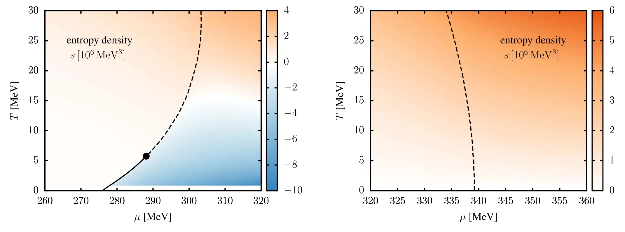
Figure 11.Entropy density for the 3d flat regulator (left panel) and 3d mass-like regulator (right panel) close to the zero temperature chiral phase boundary obtained in the QM model in LPA [159],where the solid and dashed lines denote the first-order phase transition and the crossover,respectively,and the black dot stands for the CEP.The blue region shows a negative entropy density.The plots are adopted from [159].
However,very recently another research in [159]finds that the back-bending behavior of the chiral phase boundary at large chemical potential has another different origin.It is found that the appearance of the back-bending behavior depends on the employed regulator[159].In figure 11 results of the chiral phase boundary and the entropy density obtained with two different regulators are compared.The left panel corresponds to the usually used 3d flat or optimized regulator,see equations (12) and (88),and the right is obtained with a 3d mass-like regulator,see [159]for more details.The same truncation,i.e.the local potential approximation (LPA),is used in both calculations.It is observed that the usually used flat (Litim) regulator results in a back-bending of the chiral phase line at large chemical potential,which is also accompanied by a region of negative entropy density in the chirally symmetric phase,as shown by the blue area in the left panel of figure 11.On the contrary,in the right panel one finds that the chiral phase line shows no back-bending behavior and the entropy density stays positive if a mass-like regulator is used.See [159]for a more detailed discussion.
In heavy-ion collisions since the incident nuclei do not carry the strangeness,the produced QCD matter after collisions is of strangeness neutrality,that is,the strangeness density nSis vanishing.Usually,the condition of strangeness neutrality requires that the chemical potential of strangeness μSin equation(145)is nonvanishing with μB≠0[140,141].The influence of the strangeness neutrality on the phase boundary is investigated in [140],which is presented in figure 12.One can see in comparison to the case of μS=0,the phase boundary moves up slightly due to the strangeness neutrality.In other words,the curvature of the phase boundary is decreased a bit by the condition of strangeness neutrality,see section 4.6 for more discussions about the curvature of the phase boundary.
3.2.4.Equation of state.From the effective action in equation (119) or (140),one is able to obtain the thermodynamic potential density,as follows
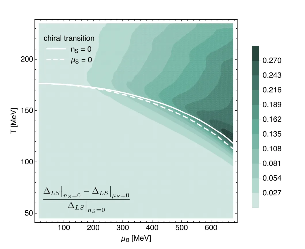
Figure 12.Phase diagram of the Nf=2+1 flavor QM model in the T–μB plane obtained in [140],where the phase boundaries in the regime of crossover for the two cases: μS=0 and the strangeness neutrality nS=0 are compared.The color stands for the relative error of the reduced condensate (see section 4.5) for the two cases.The plot is adapted from [140].
where ΦEoMdenotes the fields on the equations of motion.Then the pressure and the entropy density read

and
Moreover,the trace anomaly that is also called the interaction measure is given by
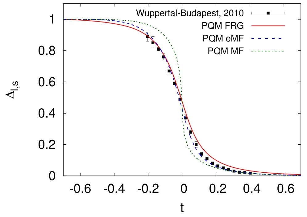
Figure 13.Reduced chiral condensate as a function of the reduced temperature in the Nf=2+1 flavor QM model obtained in [110].The fRG result (red solid line) is compared with the lattice result[160]as well as the mean-field ones.The plot is adopted from[110].
where the energy density reads
with the number density for quark of flavor f
In figure 13 the reduced condensate,see equation (229)and the relevant discussions in section 4.5,is shown as a function of the reduced temperature t=(T-Tpc)/Tpcobtained in [110],where Tpcdenotes the pseudocritical temperature for the chiral crossover.The fRG calculations are in agreement with the lattice simulations [160].Furthermore,the mean-field results are also presented for comparison,where those labelled with ‘eMF’ and ‘MF’ are obtained by taking into account or not the fermionic vacuum loop contribution in the calculations,respectively,and see,e.g.[104]for more discussions.In figure 14 the pressure and the trace anomaly in the Nf=2+1 flavor QM model obtained in[110]are shown as functions of the reduced temperature.The fRG results are compared with the lattice results [161,162],and it is observed that the fRG results are consistent with the lattice results from the Wuppertal–Budapest collaboration(WB),except that the trace anomaly from fRG is a bit larger than that from WB in the regime of high temperature with t ≿0.3.Moreover,the mean-field results as well as those including a contribution of the thermal pion gas,are also presented for comparison.
The equations of state in figure 14 are obtained in fRG within the local potential approximation,where the RG-scale dependence only enters the effective potential in equation (119).The equations of state are also calculated beyond the LPA approximation in[118].The relevant results are presented in figure 15.In the calculations,the wave function renormalizations for the mesons and quarks,and the RG scale dependence of the Yukawa coupling are taken into account.In figure 15 the results beyond LPA are in comparison to the lattice and LPA results.One can see that the trace anomaly is decreased a bit beyond LPA in the regime of T ≿1.1Tc.In figure 16 the influence of the strangeness neutrality on the isentropes is presented obtained in[140].It is found that,in comparison to the case of μS=0,the isentropes with nS=0 move towards the r.h.s.a bit,and their turning around in the regime of crossover becomes more abrupt.Moreover,isentropes obtained from the Taylor expansion and the grid method for the effective potential are compared,and consistent results are found [163].
Note that calculations of the equations of state at high baryon densities within the fRG approach have also made progress recently,see,e.g.[88,164,165],and the obtained EoS has been employed to study the phenomenology of compact stars [164,165].
3.2.5.Baryon number fluctuations.Differentiating the pressure in equation (156) with respect to the baryon chemical potential n times,one is led to the nth order generalized susceptibility of the baryon number,i.e.
which is also related to the nth order cumulant of the net baryon number distributions,that is,
with δNB=NB-〈NB〉.Here P(NB) denotes the probability distribution of the net baryon number,which can be calculated theoretically from the canonical ensemble with an imaginary chemical potential,and see,e.g.[115,142]for a detailed discussion.In experimental measurements,since neutrons are difficult to detect,the net proton number distribution is measured,as a proxy for the net baryon number distribution,and see,e.g.[22]for more details.Evidently,〈NB〉 is the ensemble average of the net baryon number.
The relations between the generalized susceptibilities in equation (161) and the cumulants in equation (162) for the lowest four orders read
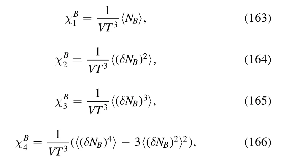
which leaves us with the experimental observables as follows
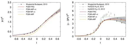
Figure 14.Pressure (left panel) and trace anomaly(right panel) as functions of the reduced temperature in the Nf=2+1 flavor QM model obtained in [110].The fRG results are in comparison to the lattice [161,162]and mean-field results.The plots are adopted from [110].
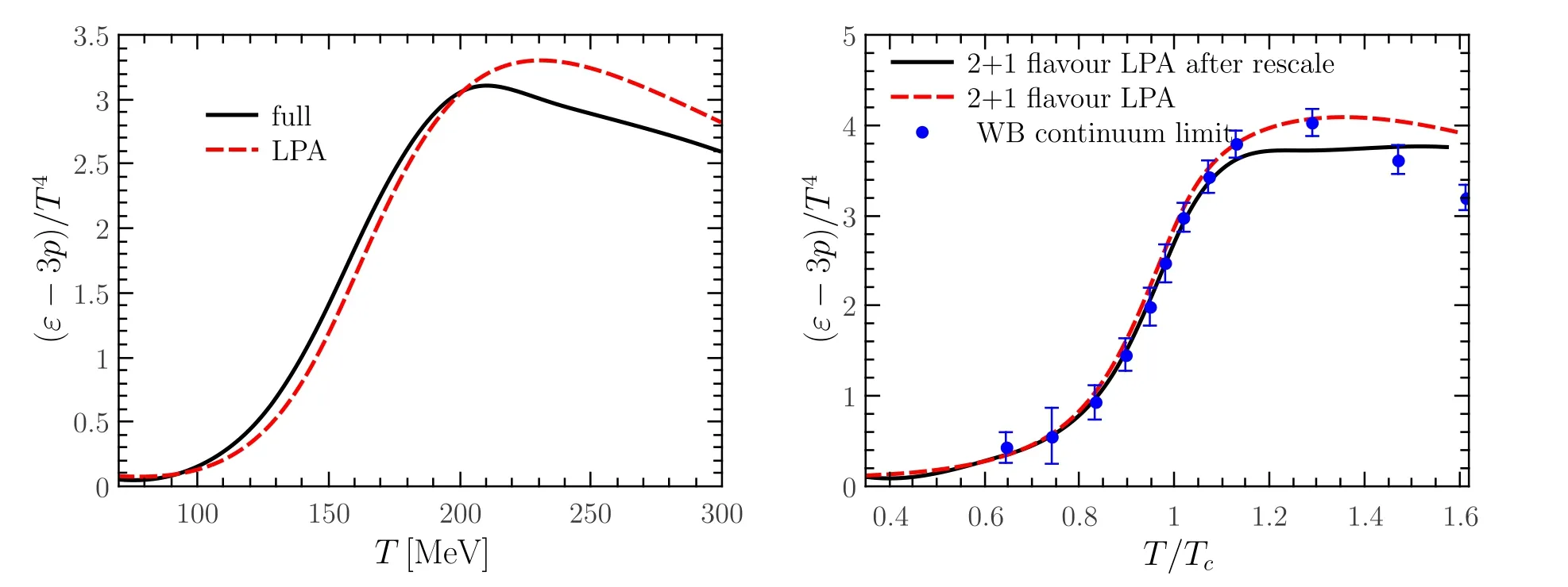
Figure 15.Left panel: Trace anomaly of the Nf=2 QM model as a function of the temperature.Here the LPA result is compared with that beyond LPA,denoted by ‘full’,in which the wave function renormalizations for the mesons and quarks,the RG scale dependence of the Yukawa coupling are taken into account.Right panel: Trace anomaly of the Nf=2+1 QM model obtained beyond LPA (labelled with‘LPA after rescale’)as a function of the temperature,in comparison to the LPA result[110]and the lattice result from Wuppertal–Budapest collaboration [162].Plots are adopted from [118].
Here M,σ2,S,к stand for the mean value,the variance,the skewness,and the kurtosis of the net baryon or proton number distributions.In the same way,calculations can also be extended to the hyper-order baryon number fluctuations,i.e.χBn>4[104,150,166–168].The relations between the hyperorder susceptibilities and the cumulants are given by [150]
It is more convenient to adopt the ratio between two susceptibilities of different orders,say
where the explicit volume dependence is removed.The baryon number fluctuations as well as fluctuations of other conserved charges,e.g.the electric charge and the strangeness,and correlations among these conserved charges,have been widely studied in the literature.For lattice simulations,see,e.g.[5–7,9–11,15].Investigations of fluctuations and correlations within the fRG approach to LEFTs can be found in,e.g.[99,101,118,119,127,138,140,141,143,147,150,168,169],and within the mean-field approximations in,e.g.[104,167,170–172].For the relevant studies from DSEs,see,e.g.[173,174].Remarkably,recently QCD-assisted LEFTs with the fRG approach have been developed and used to study the skewness and kurtosis of the baryon number distributions[118,119,127],the baryon-strangeness correlations[140,141],and the hyper-order baryon number fluctuations [150].
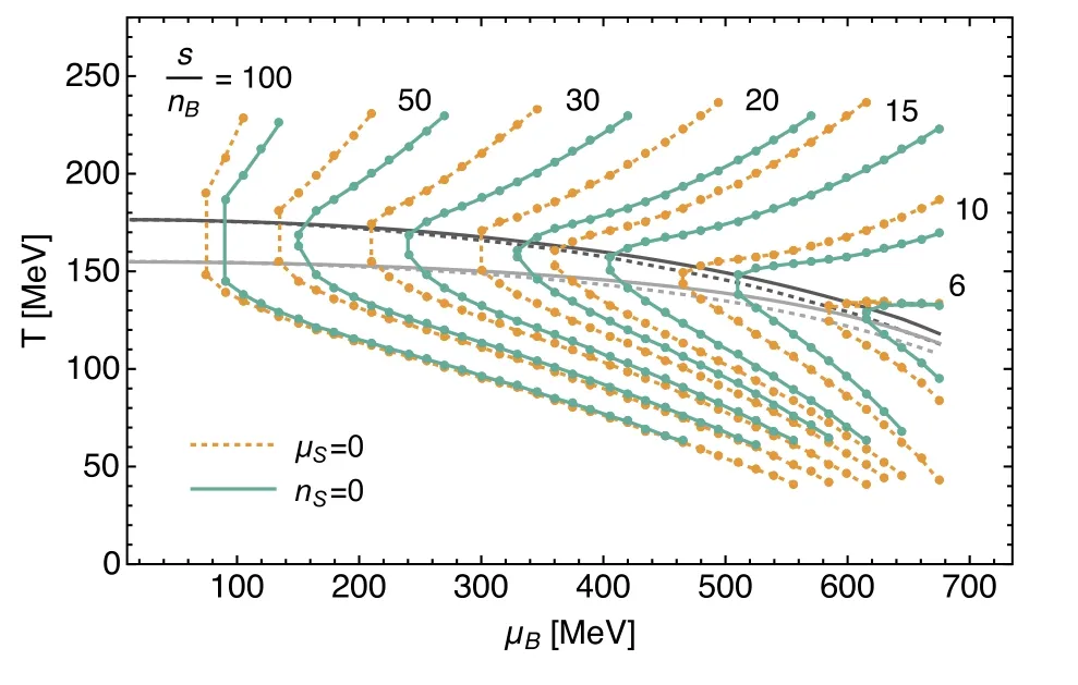
Figure 16.Isentropes for different ratios of s/nB in the phase diagram in the Nf=2+1 flavor QM model were obtained in [140].Two cases with μS=0 and the strangeness neutrality nS=0 are compared.The black and gray lines stand for the chiral and deconfinement crossover lines,respectively.The plot is adapted from [140].
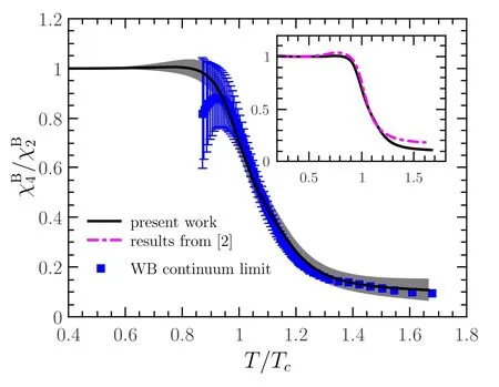
Figure 17.Kurtosis of the baryon number distributions as a function of the temperature obtained within the fRG approach to LEFTs[127].In the calculations,the frequency dependence for the quark wave function renormalization is taken into account,and the relevant results (black solid line) are compared with those without the frequency dependence (pink dashed line) in [119].The continuumextrapolated lattice results from the Wuppertal–Budapest collaboration [6]are also presented for comparison.The plot is adapted from [127].
In figure 17 the kurtosis of the baryon number distributions is shown as a function of the temperature at vanishing chemical potential.In the calculations the frequency dependence of the quark wave function renormalization is taken into account[127],whose contribution to the flow of the effective potential is shown schematically in figure 18.It is found that a summation for the quark external frequency is indispensable to the Silver Blaze property at finite chemical potential,see [127]for a more detailed discussion.From figure 17,one can see that the summation for the external frequency of the quark wave function renormalization improves the agreement between the fRG results and the lattice ones.
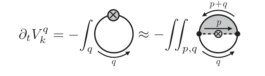
Figure 18.Schematic diagram of the frequency dependence of the quark anomalous dimension to the flow equation of the effective potential.The gray area stands for the contribution of the quark anomalous dimension,where a summation for the quark external frequency has been done.The plot is adapted from [127].
In figure 19 the fourth-,sixth-,and eighth-order baryon number fluctuations divided by the quadratic one are shown as functions of the temperature at vanishing baryon chemical potential.The fRG results [150]are compared with lattice results from the HotQCD collaboration [9,10,15]and the Wuppertal–Budapest collaboration (WB) [11].It is observed that the fRG results are in quantitative,qualitative agreement with the WB and HotQCD results,respectively.In figure 20 the baryon number fluctuations of different orders,RB31,RB42,RB51,RB62,RB71and RB82,are shown as functions of the temperature with several different values of the baryon chemical potential from 0 to 400 MeV.One finds that the dependence of fluctuations on the temperature oscillates more pronouncedly with the increasing order of cumulants.Moreover,with the increase of the baryon chemical potential the chiral crossover grows sharper,which leads to an increase in the magnitude of fluctuations significantly.
In the left panel of figure 21 the kurtosis of the baryon number distributions is depicted in the phase diagram [150].The black dashed line denotes the chiral phase boundary in the crossover regime.The green dotted line stands for the chemical freeze-out curve obtained from the STAR freeze-out data [175],see [150]for a more detailed discussion.One can see that there is a narrow blue area near the phase boundary with μB≿300 MeV,which indicates that the kurtosis becomes negative in this area.Moreover,it is found that with the increase of the baryon chemical potential,the freezeout curve moves towards the blue area firstly,and then deviates from it a bit at large baryon chemical potential.The skewness of the baryon number distributions as a function of the collision energy calculated in the fRG approach is presented in the right panel of figure 21 [150],which is in comparison to the STAR data of the skewness of the netproton number distributions Rp32with centrality 0%–5% [42].It is found that the fRG results are in good agreement with the experimental data except for the two lowest energy points,which is attributed to the fact that other effects,e.g.volume fluctuations [176–178],the global baryon number conservation [179–181],become important when the beam collision energy is low.
In figure 22 baryon number fluctuations RB42,RB62,RB82,RB31,RB51,and RB71are shown as functions of the collision energy obtained within the fRG approach [150],where the chemical freeze-out curve obtained from STAR data as shown in the left panel of figure 21 is used.The fRG results are compared with experimental data of the kurtosis of the netproton number distributions Rp42with centrality 0%–5% [42],and the sixth-order cumulant Rp62with centrality 0%–10%[43].A non-monotonic dependence of the kurtosis RB42on the collision energy is also observed in the fRG calculations,which is consistent with the experimental measurements of Rp42.Moreover,it is found that this non-monotonicity arises from the increasingly sharp crossover with the decrease of the collision energy,which is also reflected in the heat map of the kurtosis in the phase diagram in the left panel of figure 21.The fRG results of RB62are also qualitatively consistent with the experimental data of Rp62.
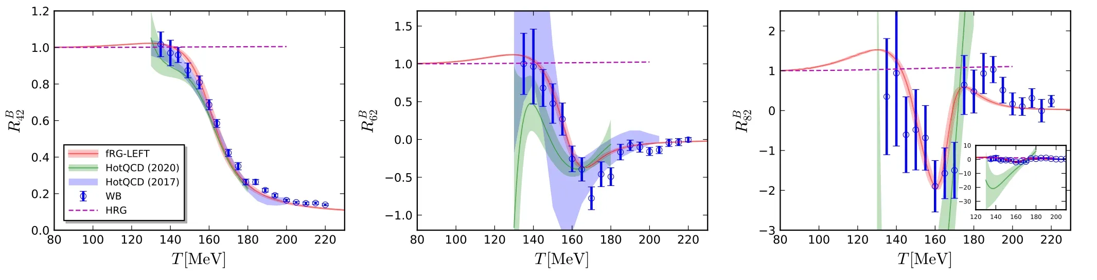
Figure 19.Baryon number fluctuations RB42(left panel),RB62(middle panel),and RB82(right panel) as functions of the temperature at μB=0,obtained within the fRG approach to a QCD-assisted LEFT in [150].The fRG results are compared with lattice results from the HotQCD collaboration[9,10,15]and the Wuppertal–Budapest collaboration[11].The inlay in the right panel shows the zoomed-out view of RB82.The plots are adopted from [150].
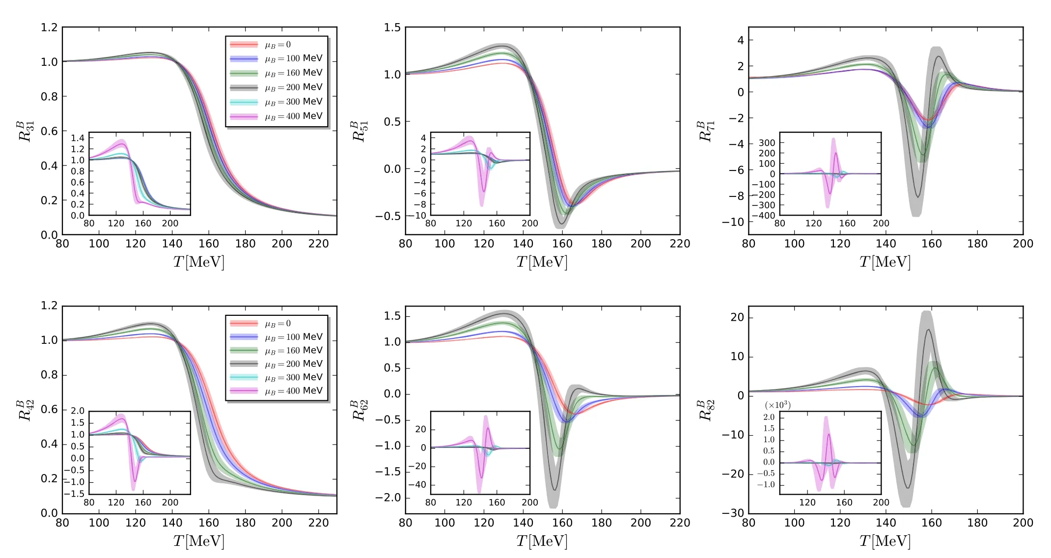
Figure 20.Baryon number fluctuations RB31 (top-left),RB42 (bottom-left),RB51 (top-middle),RB62 (bottom-middle),RB71 (top-right) and RB82(bottom-right) as functions of the temperature with several different values of the baryon chemical potential,obtained within the fRG approach to a QCD-assisted LEFT in [150].The inlays in each plot show the zoomed-out views.The plots are adopted from [150].
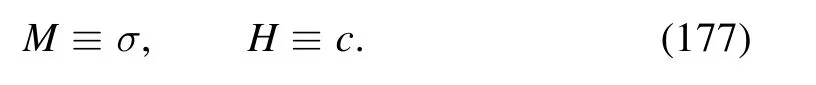
In figure 23 the full results of the baryon number fluctuations RB42and RB62are compared with those of Taylor expansion for the baryon chemical potential up to the eighth and tenth orders,which can be used to investigate the convergence properties of the Taylor expansion for the baryon chemical potential.For the two values of the temperature,T=155 MeV and 160 MeV,it is found that the full results deviate from those of Taylor expansion significantly with μB/T ≿1.2–1.5.The oscillating behavior of the full results at large baryon chemical potential is not captured by the Taylor expansion,which hints that the convergence radius of the Taylor expansion for the baryon chemical potential might be restricted by some singularity,e.g.the Yang–Lee edge singularity,and see,e.g.[182–185]for more discussions.

Figure 21.Left panel:Kurtosis of the baryon number distributions R4B2 (T,μB)in the phase diagram,obtained within the fRG approach to a QCD-assisted LEFT in [150].The black dashed line stands for the chiral phase boundary in the crossover regime obtained from QCD calculations[18].The green dotted line denotes the chemical freeze-out curve.Right panel:Skewness of the baryon number distributions as a function of the collision energy,obtained within the fRG approach to a QCD-assisted LEFT in[150].The fRG results are compared with the experimental measurements of the skewness of the net-proton number distributions Rp32 with centrality 0%–5% [42].The plots are adopted from [150].
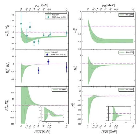
Figure 22.Baryon number fluctuations RB42 (top-left),RB62 (middleleft),RB82 (bottom-left),RB31 (top-right),RB51 (middle-right),RB71(bottom-right) as functions of the collision energy,obtained within the fRG approach to a QCD-assisted LEFT in [150].Experimental data of the kurtosis of the net-proton number distributions Rp42 with centrality 0%–5% [42],and the sixth-order cumulant Rp62 with centrality 0%–10%[43]are presented for comparison.The plots are adopted from [150].
We close this subsection with a discussion about the correlation between the baryon number and the strangeness,i.e.
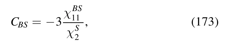
which is calculated within the fRG approach in [141].There,the influence of the strangeness neutrality on CBSis investigated,and the relevant results are presented in figure 24.One can see that the correlation between the baryon number and the strangeness is suppressed by the condition of the strangeness neutrality.
3.2.6.Critical exponents.According to the scaling argument,when a system is in the critical regime,its thermodynamic potential density can be decomposed into a sum of a singular and a regular part [66],viz.,

where of,the singular part satisfies the scaling relation to the leading order as follows
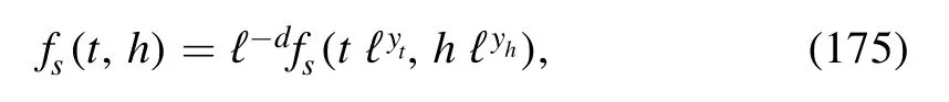
with a dimensionless rescaling factor ℓ and the spatial dimension d.In equations (174) and (175) t and h stand for the reduced temperature and magnetic field,respectively.They are given by
where Tcis the critical temperature in the chiral limit,and T0and c0are some normalization values for the temperature T and the strength of the explicit chiral symmetry breaking c as shown in equation (119),respectively.In the following,the order parameter will be denoted as the magnetization density,and c as the magnetic field strength,i.e.
The scaling relation in equation (175) leaves us with a set of scaling relations for various critical exponents,see [66,186],such as,
Figure 23.Full results of the baryon number fluctuations RB42 (upper panels) and RB62 (lower panels) as functions of μB/T with two fixed values of the temperature,in comparison to the results of Taylor expansion up to order of χ8B(0)(left panels)and χ1B0 (0)(right panels).Both results are obtained within the fRG approach to a QCD-assisted LEFT in [150].The plots are adopted from [150].
The critical behavior of the order parameter is described by the critical exponents β and δ,which read

with t<0,and

Moreover,one has the susceptibility of the order parameter χ and the correlation length ξ,which scale as

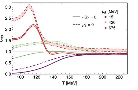
Figure 24.Correlation between the baryon number and the strangeness CBS as a function of the temperature with several different values of the baryon chemical potential,obtained within the fRG approach in [141].Two cases with μS=0 (dashed lines) and the strangeness neutrality nS=0(solid lines)are compared.The plot is adapted from [141].
Recently,the pseudo-spectral method of the Chebyshev expansion for the effective potential has been used to calculate the critical exponents [151].In the Nf=2 QM model within the fRG approach,the critical exponents for the 3d O(4) and Z(2) symmetry universality classes,which correspond to the black dashed O(4)phase transition line and the red dashed Z(2)phase transition line as shown in figure 9 respectively,are calculated with the Chebyshev expansion of the effective potential.Both the LPA and LPA′ approximations are used in the calculations.In the LPA′approximation a field-dependent mesonic wave function renormalization is taken into account.The relevant results are shown in table 1,which are also compared with results of critical exponents from other approaches,e.g.Taylor expansion of the effective potential[186–190]and the grid method[191]within the fRG approach,the derivative expansions (DE) up to orders of O (∂4)and O (∂6)with the fRG approach [192,193],the conformal bootstrap for the 3d conformal field theories(CFTs) [194,195],Monte Carlo simulations [196],and the d=3 perturbation expansion [197].In the meantime,the mean-field values of the critical exponents are also shown in the last line of table 1.
In figure 25 the critical exponent β for the 3d O(4)and Z(2) symmetry universality classes extracted from different ranges of temperature is shown,which is obtained with the Chebyshev expansion for the effective potential in the fRG[151].It is found that only when the temperature is very close to the critical temperature,say |T-Tc|≾0.01 MeV,the fRG results of both the O(4) and Z(2) symmetry universality classes are consistent with the conformal bootstrap results.This indicates that the size of the critical region is extremely small,far smaller than~1 MeV.Similar estimates for the size of the critical region are also found in,e.g.[98,186,198,199].
4.QCD at finite temperature and density
In this section,we would like to present a brief review on recent progress in studies of QCD at finite temperature and densities within the fRG approach to the first-principle QCD,which are mainly based on the work in[18,62].The relevant fRG flows at finite temperature and densities there have been developed from the counterparts in the vacuum in [59,60].Furthermore,these flows are also built upon the state-of-theart quantitative fRG results for Yang–Mills theory in the vacuum [56]and at finite temperature [57],QCD in the vacuum [58,61].
In the following,we focus on the chiral phase transition.As mentioned above,the QCD phase transitions involve both the chiral phase transition and the confinement-deconfinement phase transition.In fact,related subjects of the deconfinement phase transition,such as the Wilson loop,the Polyakov loop,the flows of the effective action of a background gauge field,the relation between the confinement and correlation functions,etc,have been widely studied within the fRG approach to Yang–Mills theory and QCD.Significant progress has been made in relevant studies,see [55]for a recent overview,and also e.g.[70,108,200–215].
4.1.Propagators and anomalous dimensions
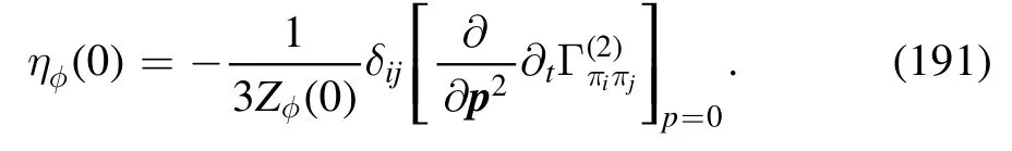
The flow equations of inverse propagators are obtained by taking the second derivative of the Wetterich equation in equation (80) with respect to respective fields.The resulting flow equations of the inverse quark,gluon and meson propagators are shown diagrammatically in figure 26.Making appropriate projections for these flow equations,one is able to arrive at the flow of the wave function renormalization ZΦ,kas shown in equation (49) for a given field Φ,which includes nontrivial dispersion relation for the field,and is more conveniently reformulated as the anomalous dimension as follows
The quark two-point correlation function defined in equation (84),see also equation (A24),reads
where ΦEoMdenotes the fields in equation (62) on their respective equations of motion,that are vanishing except the σ field and the temporal gluon field A0.Note that the minus sign on the r.h.s.of equation (183),while not appearing in equation (A24),is due to the fact that the right derivative is used in equation (A24).Moreover,the quark chemical potentials in equation(48)have been assumed to be vanishing in equation (183).Apparently,the quark wave function renormalization and mass are readily obtained by projecting equation (183) onto the vector and scalar channels,respectively,which read
where the trace runs only in the Dirac space.Neglecting the dependence of the quark wave function renormalization on the spacial momentum p,one arrives at the quark anomalous dimension as follows
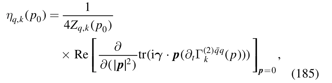
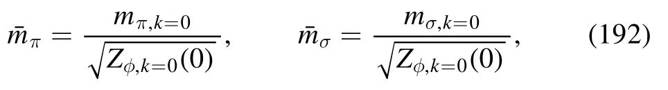
where the computation is done at p=0,and p0is a small,but nonvanishing frequency.The nontrivial choice of p0and the fact that the expression in the square bracket in equation(185)is complex-valued at nonzero chemical potentials,are both related to constraints from the Silver-Blaze property for the correlation functions at finite chemical potentials,and see,e.g.[18,119,120,127,216]for more details.In equation(185)Re denotes that the real part of the expression in the square bracket is adopted.Note that in equation (185)the difference between the parts of the quark wave function renormalization longitudinal and transversal to the heat bath is ignored,where the projection is done on the spacial component,and thus the transversal anomalous dimension is used.The explicit expression of ηq,kis given in equation(C1).In the left panel of figure 27,the quark wave function renormalization Zq,k=0(p0,p=0)is depicted as a function of the temperature with different values of the baryon chemical potential.
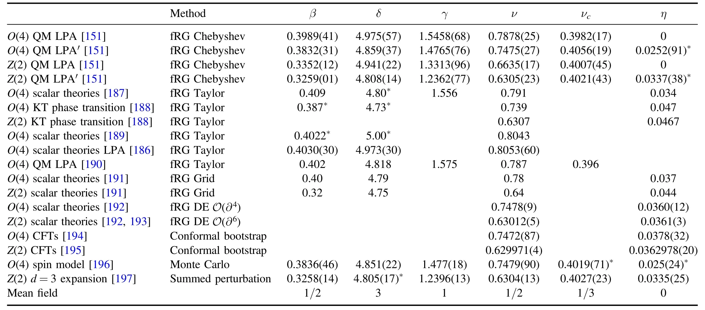
Table 1.Comparison of the critical exponents for the 3d O(4)and Z(2)symmetry universality classes from different approaches.The values with an asterisk are derived from the scaling relations in equation (178).The table is adapted from [151].
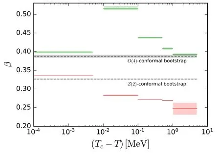
Figure 25.Critical exponent β for the 3d O(4)(green lines)and Z(2)(red lines) symmetry universality classes extracted from different ranges of the temperature,obtained within the fRG approach in[151].The conformal bootstrap results(gray dashed lines)[194,195]are also presented for comparison.The plot is adapted from [151].
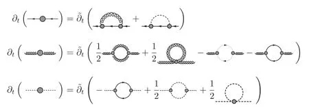
Figure 26.Diagrammatic representation of the flow equations for the inverse quark,gluon and meson propagators,respectively,where the dashed lines stand for the mesons and the dotted lines denote the ghost.
The mesonic two-point correlation functions,i.e.those of the π and σ fields,are given by
and
respectively,where the curvature masses of the mesons read

As same as the quark wave function renormalization,the thermal splitting of the mesonic wave function renormalization in parts longitudinal and transversal to the heat bath is neglected.Moreover,one has assumed a unique renormalization for both the pion and sigma fields,viz.,Zφ,k=Zπ,k=Zσ,k.The validity of these approximations has been verified seriously in[148].The anomalous dimension of mesons at vanishing frequency p0=0 and a finite spacial momentum p is given by

Two cases are of special interest: one is the choice p2=k2,i.e.ηφ(0,k),which captures the most momentum dependence of the mesonic two-point correlation functions,and thus is usually used in the r.h.s.of flow equations involving mesonic degrees of freedom,for more detailed discussions see [18].The anomalous dimension ηφ(0,k) leaves us with the renormalization constant defined as follows
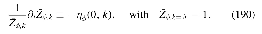
In the right panel of figure 27,is depicted as a function of the temperature with different values of the baryon chemical potentials.The other is the case p=0,and equation (189) is reduced the equation as follows
The related wave function renormalization Zφ,k(0) is used to extract the renormalized meson mass as
whereandare approximately equal to their pole masses,respectively.The explicit expressions for equations(191)and(189)are presented in equations(C2)and(C3),respectively.
For the ghost anomalous dimension,one extracts it from the relation as follows
where(p)denotes the momentum-dependent ghost wave function renormalization in QCD with Nf=2 flavors in the vacuum obtained in[61].Note that the ghost propagator is found to be very insensitive to the effects of finite temperature as well as the quark contributions for Nf=2 and Nf=2+1 flavors,see e.g.[57].
The gluon anomalous dimension is decomposed into a sum of three parts,as follows

where the first term on the r.h.s.denotes the gluon anomalous dimension in the vacuum,and the other two terms stand for the medium contributions to the gluon anomalous dimension from the glue (gluons and ghosts) and quark loops,respectively.The vacuum contribution in equation (194) is further expressed as
where the two terms on the r.h.s.denote the contributions from the light quarks of Nf=2 flavors and the strange quark.
The former one is inferred from the gluon dressing function(p)for the Nf=2 flavor QCD in [61],which reads
Figure 27.Quark(left panel,Zq)and mesonic(right panel,Z)wave function renormalizations of Nf=2+1 flavor QCD obtained in the fRG with RG scale k=0,as functions of the temperature with different values of the baryon chemical potential.The plot is adapted from [18].
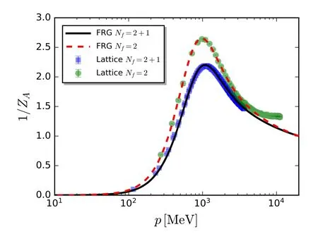
Figure 28.Gluon dressing functions 1/ZA(p) of Nf=2 and Nf=2+1 flavor QCD in the vacuum as functions of the momentum,where the fRG results are in comparison to lattice calculations of Nf=2 flavors [217]and Nf=2+1 flavors[218,219].The plot is adapted from [18].
The explicit expressions ofin equation (194) andequation (196),which is also in quantitative agreement with the lattice result in [217].Note that the gluon dressing of Nf=2+1 flavors here is a genuine prediction,which is in good agreement with the respective lattice results [218,219].In figure 29 both the gluon dressing function and the gluon propagator of Nf=2+1 flavors are presented.The calculated gluon dressing functions at finite temperature and baryon chemical potential in fRG are shown in figure 30.In the left panel of figure 30 several different values of temperature are chosen with μB=0,and it is found that the gluon dressing function 1/ZAdecreases with the increase in temperature.In the right panel,several different values of μBare adopted while with T=150 MeV fixed.It is observed that the dependence of the gluon dressing function on the baryon chemical potential is very small.The gluon dressing functions at finite temperature obtained in fRG are compared with the relevant lattice results from [220]in figure 31,where several different values of temperature are chosen.One can see that the gluon dressing at finite temperature in fRG is comparable to that of lattice QCD.
4.2.Strong couplings
The quark-gluon coupling in equation (53),the ghost-gluon coupling in equation (54),and the three-gluon or four-gluon coupling in equation(50),etc,are consistent with one another in the perturbative regime of high energy,due to the Slavnov–Taylor identities (STIs) resulting from the gauge symmetry.However,when the momenta or the RG scale are decreased to k ≾1–3 GeV,the gluon mass gap begins to affect the running of strong couplings,and also the transversal strong couplings can not be identified with the longitudinal ones via the modified STIs,see,e.g.[56,215,222,223]for more details.Consequently,different strong couplings deviate from one another in the low energy regime of k ≾1–3 GeV [56–58,61],and thus it is necessary to distinguish them by adding appropriate suffixes.The couplings of the purely gluonic in equation (195) can be found in equations (C4)–(C6).Moreover,the in-medium contribution to the gluon anomalous dimension resulting from the glue sector,i.e.the second term on the r.h.s.of equation (194),is taken into account in equation (C7).
In figure 28 the gluon dressing functions 1/ZA(p) of Nf=2 and Nf=2+1 flavor QCD in the vacuum are shown.The fRG and lattice results are presented.Here the fRG gluon dressing of Nf=2 flavors is inputted from [61],as shown in sector read
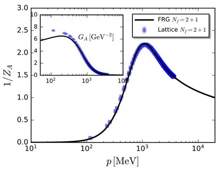
Figure 29.Gluon dressing function 1/ZA(p) and the gluon propagator GA=1/[ZA(p)p2](inlay) as functions of momenta for QCD of Nf=2+1 flavors in the vacuum,where the fRG results denoted by the black lines are compared with the continuum extrapolated lattice results by the RBC/UKQCD collaboration,see e.g.[218,219,221].For the fRG results,the momentum dependence is given by p2=k2.The plot is adapted from [18].
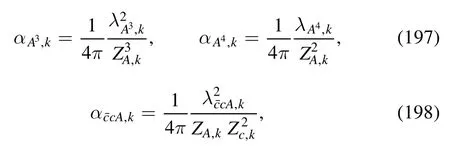
whereλA3,k,λA4,kanddenote the three-gluon,fourgluon,ghost-gluon dressing functions,respectively,as shown in equations(A42),(A48),(A36).The couplings of the matter sector read
where the light-quark-gluon coupling and the strange-quarkgluon coupling have been distinguished.From the calculated results in,e.g.[59,61],it is reasonable to adopt the approximation as follows

The flow equation of the quark-gluon vertex is presented in the first line of figure 32.Projecting onto the classical tensor structure of the quark-gluon vertex,denoted by
one is led to the flow of the quark-gluon coupling as follows
where the trace sums over the Dirac and color spaces,and{p}stands for the set of external momenta for the vertex.Here≡is used.In equation (202) the flow of quarkgluon vertex,i.e.the r.h.s.of the first line in figure 32,is denoted by
with
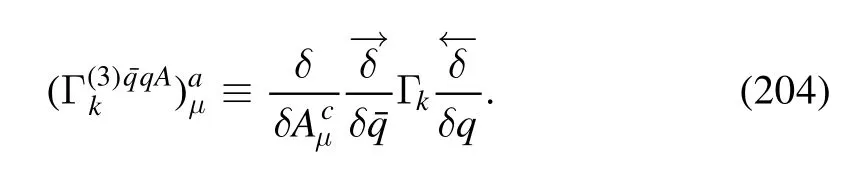
Note that besides the classical tensor structure of the quarkgluon vertex in equation (201),some nonclassical tensor structures also play a sizable role in the dynamical breaking of the chiral symmetry [58,61,224],see,e.g.[18]for more detailed discussions.From equation (202) one formulates the flow of the light-quark–gluon coupling as
where the second term on the r.h.s.corresponds to the two diagrams on the r.h.s.of the flow equation for the quark-gluon vertex as shown in the first line of figure 32,and the last term to the last diagram,which arises from the quark-gluon,quarkmeson fluctuations,respectively.For the strange-quark–gluon coupling,one has
where the contribution from the strange-quark–meson interactions is neglected,that is reasonable due to relatively larger masses of the strange quark and strange mesons.The explicit expressions in equations (205) and (206) can be found in equations (C9) and (C10).
In the same way,the flow equation of the three-gluon coupling,gA3,k≡λA3,k,is readily obtained from the flow of the three-gluon vertex in the second line of figure 32.The flow of the three-gluon coupling is decomposed into a sum of the vacuum part and the in-medium contribution,as follows

where the vacuum part,i.e.the first term on the r.h.s.is computed in [59],and the second term is identified with the in-medium contribution of the quark-gluon coupling,to wit,
In figure 33 the light-quark–gluon coupling,the strangequark–gluon coupling,and the three-gluon coupling are depicted as functions of the RG scale for several different values of the temperature.It is observed that different couplings are consistent with one another in the regime of k ≿3 GeV,while deviations develop in the nonperturbative or even semiperturbative scale.Moreover,one can see that the strong couplings decrease with the increasing temperature.
4.3.Dynamical hadronization,four-quark couplings and Yukawa couplings
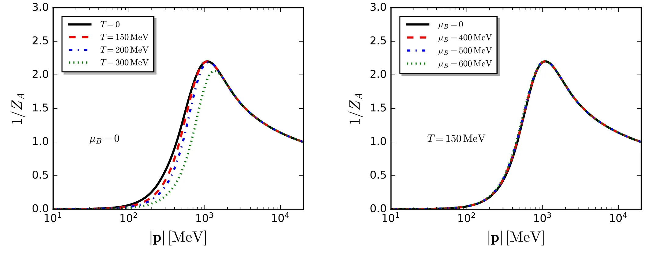
Figure 30.Gluon dressing function 1/ZA of the Nf=2+1 QCD as a function of spatial momenta |p| with several different values of temperature (left panel) and baryon chemical potential (right panel),where the Matsubara frequency p0 is chosen to be vanishing.The identification p2=k2 is used.The plot is adapted from [18].
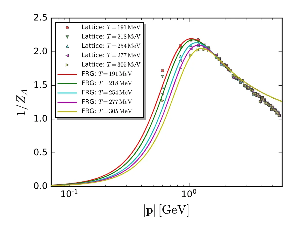
Figure 31.Gluon dressing function 1/ZA of Nf=2+1 flavors as a function of spatial momenta |p| at several values of temperature obtained in fRG,which is also compared with the lattice results of Nf=2+1+1 in [220].The plot is adapted from [18].
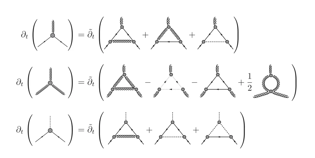
Figure 32.Diagrammatic representation of the flow equations for the quark-gluon,three-gluon,and the quark-meson vertices,respectively.
Following section 2.5,one performs the dynamical hadronization for the σ–π channel,and use
with τ=(T0,iγ5T) as shown in equation (48),whereis called the hadronization function.It is more convenient to adopt the dimensionless,renormalized hadronization function and four-quark coupling
and the renormalized Yukawa coupling,
Inserting the effective action in equation (48) into equation (80) and performing a projection on the four-quark interaction in the σ–π channel,one is left with

where
is the flow of the four-quark coupling in the σ–π channel,whose contributions have been depicted in figure 34.One can see that the contributed diagrams can be classified into three sets,which correspond to the three lines on the r.h.s.of the flow equation in figure 34.The first line is comprised of diagrams with two gluon exchanges and the second line with two meson exchanges.The last line denotes the contributions from the mixed diagrams with one gluon exchange and one meson exchange.The mixed diagrams are negligible,since the dynamics of gluons and mesons dominate in different regimes of the RG scale,as shown in figure 35.Therefore,the four-quark flow in equation (213) can be further written as
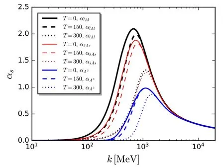
Figure 33.Quark-gluon couplings for light quarks()and strange quarks (),and the three-gluon coupling (αA3) of Nf=2+1 flavor QCD as functions of the RG scale k at several values of the temperature and vanishing baryon chemical potential.The plot is adapted from [18].
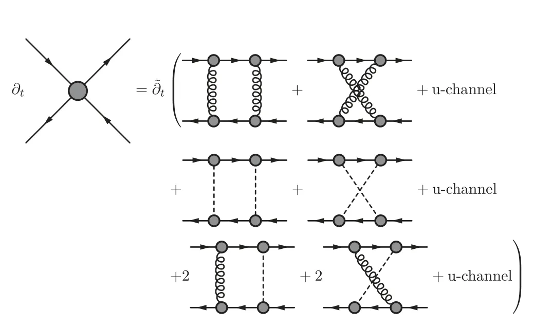
Figure 34.Diagrammatic representation of the flow equation for the four-quark vertex.The first line on the r.h.s.denotes the contributions from two gluon exchanges and the second line those from two meson exchanges.The last line stands for the contributions from the mixed diagrams with one gluon exchange and one meson exchange.
where the two terms on the r.h.s.correspond to the contributions from the two gluon exchanges and two meson exchanges,respectively.Their explicit expressions are presented in equations (C11) and (C12).In figure 35 the two terms on the r.h.s.of equation (214) and their ratios with respect to the total flow of the four-quark coupling are depicted as functions of the RG scale with T=0 and μB=0.It is observed that the flow resulting from the gluon exchange is dominant in the region of high energy,while that from the meson exchange plays a significant role in lower energy.
The dynamical hadronization is done by demanding
for every value of the RG scale k,which is equivalent to the fact that the Hubbard–Stratonovich transformation is performed for every value of k.Thus from equation (212) one arrives at the hadronization function as follows
Inserting the effective action in equation (48) into (80)and performing a projection on the Yukawa interactions between quarks and σ–π mesons,i.e.τ·φq,one is led to
with the dimensionless and renormalized pion mass as follows
Here in equation (217)
is the flow of the Yukawa coupling between the pion and quarks,which is shown in the third line of figure 32.Its explicit expression is presented in equation(C13).Therefore,by substituting the hadronization function in equation (216)into(217),one obtains the total flow of the Yukawa coupling finally.Evidently,the dynamics of resonance of quarks are stored in the interactions between quarks and mesons through dynamic hadronization.
In the left panel of figure 36,the renormalized Yukawa coupling with k=0 is shown as a function of the temperature with several different values of baryon chemical potential.It is observed that with the increase of T or μB,the Yukawa coupling decays rapidly due to the restoration of the chiral symmetry.In the right panel of figure 36,the dependence of the renormalized Yukawa coupling on the RG scale for different values of temperature is investigated.One can see that the Yukawa coupling is stable in the region of k ≿1 GeV,and the effects of temperature play a role approximately in k ≾2πT.The effective four-quark coupling in the σ–π channel can be described by the ratio[18,59],which is shown as a function of the RG scale with several different values of temperature and μB=0 in figure 37.It is observed that with the decrease of k and entering the regime of the chiral symmetry breaking,a resonance occurs in the scalar-pseudoscalar channel,which results in a rapid increase of the effective four-quark coupling.Moreover,the dependence of the effective four-quark coupling on the baryon chemical potential is shown in figure 38.One finds that the effective four-quark coupling decrease with the increasing temperature or baryon chemical potential.
4.4.Natural emergence of LEFTs from QCD
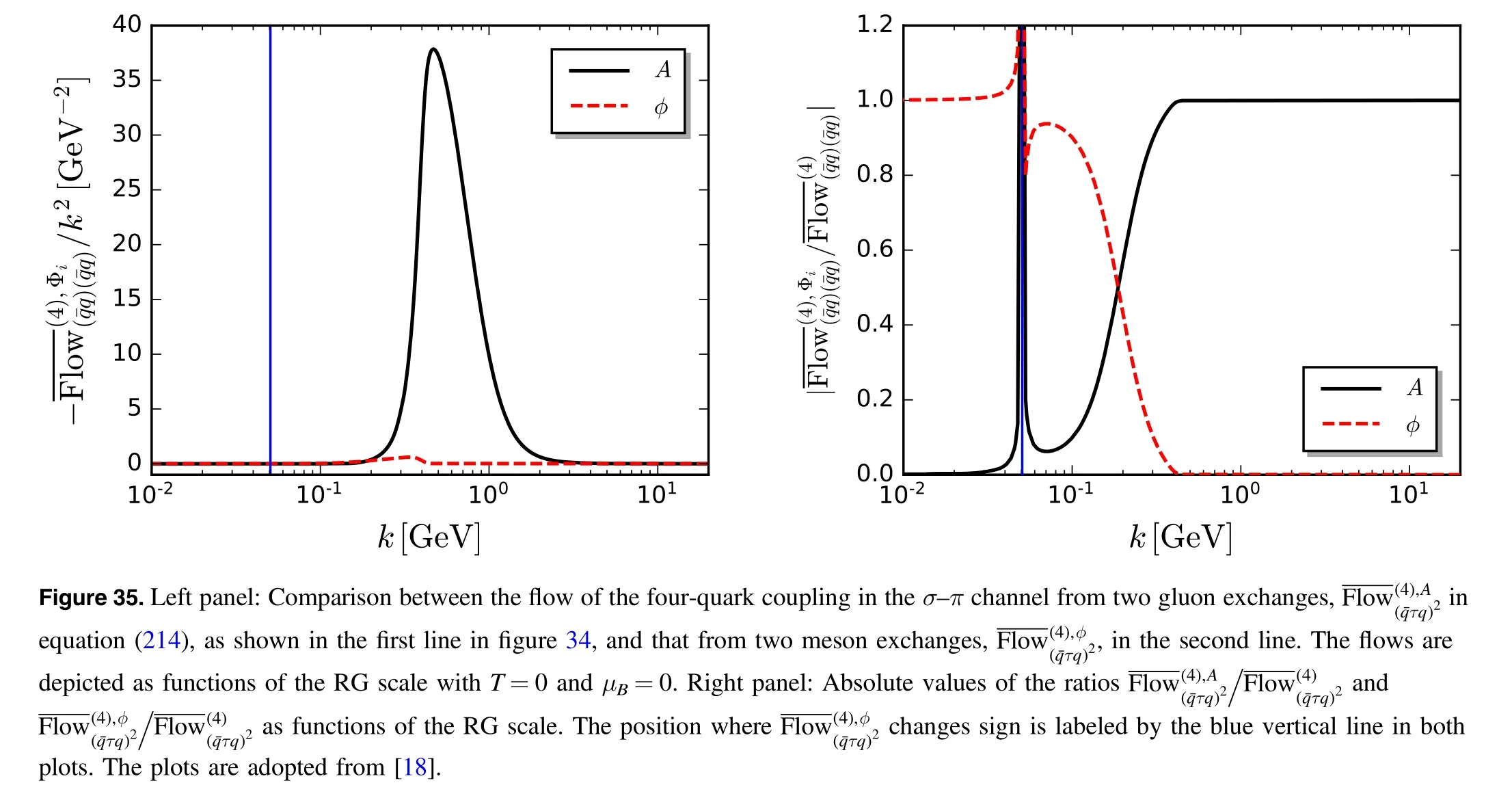
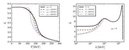
Figure 36.Left panel: Renormalized Yukawa coupling of Nf=2+1 flavor QCD at vanishing RG scale k=0 as a function of the temperature with several different values of μB obtained in fRG.Right panel:Renormalized Yukawa coupling of Nf=2+1 flavor QCD as a function of the RG scale with several different values of T and μB=0.The plots are adopted from [18].
The fRG approach to QCD with the dynamical hadronization discussed above,provide us with a method to study the transition of degrees of freedom from fundamental to composite ones.One is also able to observe a natural emergence of LEFTs from the original QCD.To that end,figure 39 shows the four-quark single gluon exchange coupling for light quarksand strange quarks,dimensionless four-quark single meson exchange couplingandas functions of the RG scale in the vacuum.Evidently,it is found that the gluonic exchange couplings are dominant in the perturbative regime of k ≿1 GeV.However,with the decrease of the RG scale the active dynamic is taken over gradually by the mesonic degrees of freedom,and one can see that the gluonic couplings and the Yukawa couplings are comparable to each other at k ≈600.In fgiure 40 dimensionless propagator gappingsfor Φi=l,s,σ,π are shown as functions of the RG scale.The gluon dressing function is also shown there for comparison.In figure 40 one observes the same information on decouplings as in figure 39,that is,as the RG scale evolves from the UV towards IR,the gluons decouple from the matter at first,then the quarks,and the mesons finally.For more related discussions see [18].
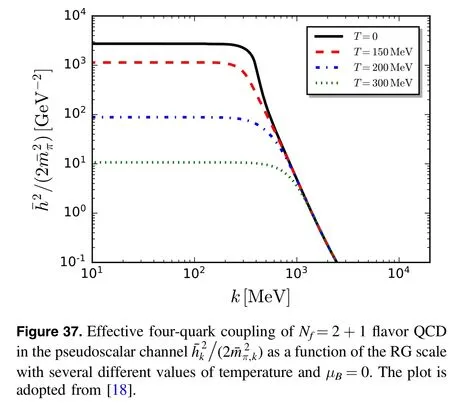
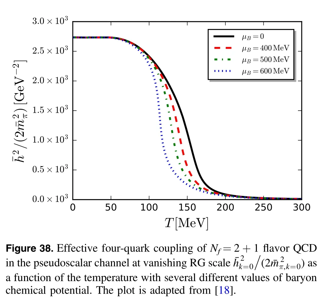

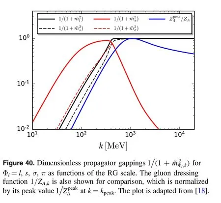
4.5.Chiral condensate
The chiral condensate of quark qi=u,d,s reads
up to a renormalization term,where no summation for the index i is assumed andis the current quark mass.Obviously,the light quark condensate is given by Δl=Δu=Δdwithml0=mu0=md0.The renormalized condensate is as follows
renders the vacuum part of the chiral condensate in equation (220) to be subtracted,where the dimensionless Δqi,Ris normalized by a constant NR,e.g.NR~fπ4.In the present fRG approach to QCD,the light quark condensate is given by
where Ω is the thermodynamic potential with the field ΦEoMbeing on is the equation of motion.From equation(48),one is led to
and
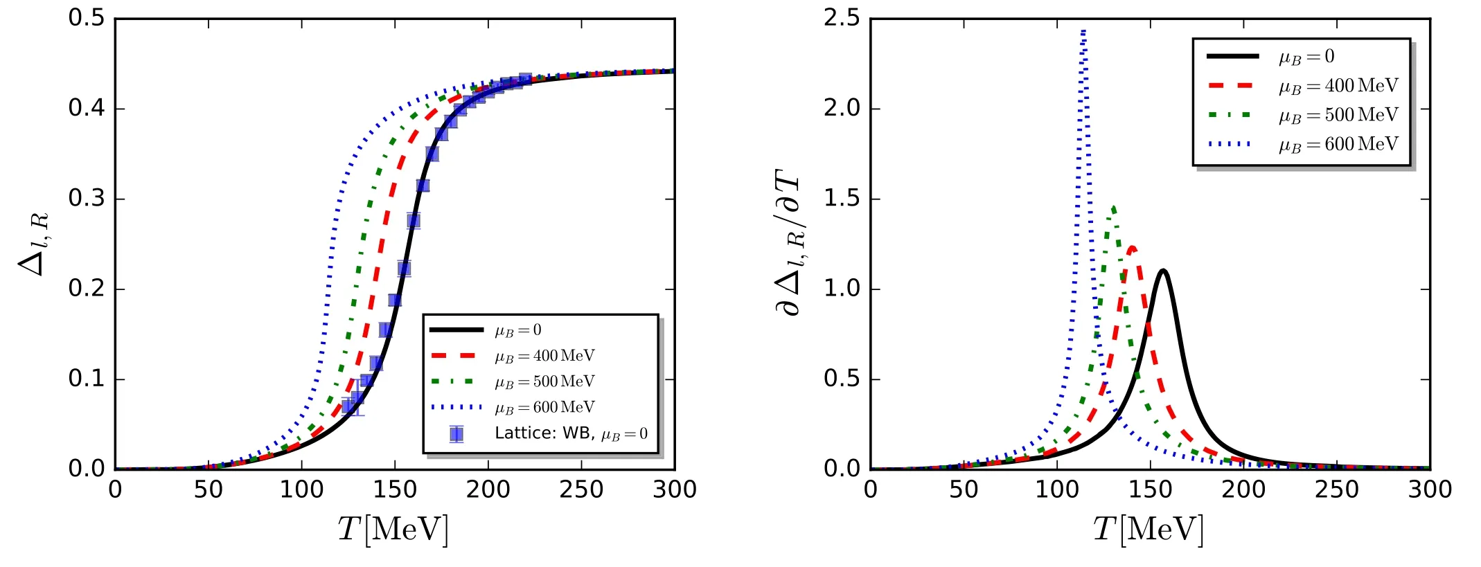
Figure 41.Left panel: Renormalized light quark chiral condensate Δl,R of Nf=2+1 flavor QCD as a function of the temperature with several different values of baryon chemical potential obtained in fRG,in comparison to the lattice results at vanishing μB[160].Right panel:Derivative of Δl,R with respect to the temperature,i.e.the thermal susceptibility of the renormalized light quark condensate,as a function of the temperature with several different values of baryon chemical potential.The plots are adopted from [18].
The reduced condensate Δl,sis defined as the weighted difference between the light and strange quark condensates as follows,
which is usually normalized with its value in the vacuum,i.e.
Similar to equation (222),one arrives at
and thus
Finally,one is led to
where one has used
In the left panel figure 41,the renormalized light quark condensate is shown as a function of the temperature with several different values of baryon chemical potential.In the case of vanishing baryon chemical potential,the fRG result is compared with the continuum extrapolated result of lattice QCD [160],and excellent agreement is found.In the right panel of figure 41,the derivative of Δl,Rwith respect to the temperature,i.e.the thermal susceptibility of the renormalized light quark condensate,is shown.The peak position of the thermal susceptibility can be used to define the pseudocritical temperature,which is found to be Tc=156 MeV for μB=0,in good agreement with the lattice result.Figure 42 shows the reduced condensate as a function of the temperature with μB=0,in comparison to the lattice simulations.One finds that for the physical current quark mass ratio,i.e.[225],the fRG results are in quantitative agreement with the lattice ones.
4.6.Phase structure
The QCD phase diagram in the plane of T and μBis shown in figure 43.The first-principle fRG results in [18]are in comparison to state-of-the-art calculations of other functional approaches,e.g.the DSE [19,20],and lattice QCD [8,12].The phase boundary in the regime of continuous crossover at small or medium μBshows the dependence of the pseudocritical temperature on the value of the baryon chemical potential.In the calculations of fRG,this pseudocritical temperature is determined by the thermal susceptibility of the renormalized light quark chiral condensate,∂Δl,R/∂T,as discussed in section 4.5.Expanding the pseudocritical temperature around μB=0,one arrives at
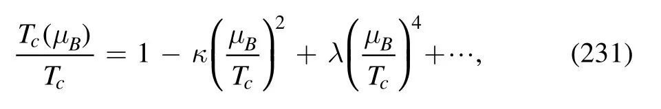
with Tc=Tc(μB=0),where the quadratic expansion coefficient к is usually called the curvature of the phase boundary.It is a sensitive measure for the QCD dynamics at finite temperature and densities.Therefore,it provides a benchmark test for functional approaches to make a comparison of the curvature at small baryon chemical potential with lattice simulations.The curvature values of the phase boundary obtained from fRG,DSE,and lattice QCD are summarized in the second line of table 2.It is found recent results of the curvature from state-of-the-art functional approaches,e.g.fRG [18],DSE [19,20],have already been compared to the lattice results.By contrast,those obtained from relatively former calculations of functional methods,e.g.[21,226,227],are significantly larger than the values of the curvature obtained from lattice simulations.
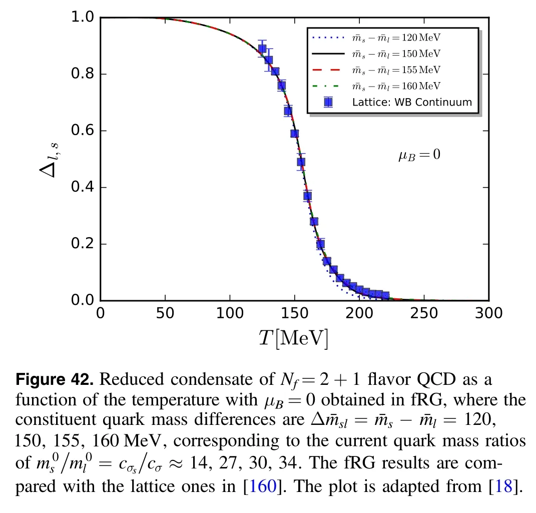
Besides the curvature of the phase boundary,another key ingredient of the QCD phase structure is the CEP of the firstorder phase transition line at large baryon chemical potential,which is currently searched for with lots of effort in experiments[22,37–43].Lattice simulations,however,are restricted in the region of μB/T ≾2–3 because of the sign problem at finite chemical potentials,and in this region,no signal of CEP is observed [17].Passing lattice benchmark tests at small baryon chemical potentials,functional approaches are able to provide relatively reliable estimates for the location of the CEP.The recent results of CEP after benchmark testing are presented in the third line of table 2,and also depicted in the phase diagram in figure 43.Remarkably,estimates of CEP from fRG and DSE converge in a rather small region at baryon chemical potentials of about 600 MeV.Note that results of [20]in table 2 are obtained without the dynamics of sigma and pion,and the relevant results are к=0.0167 and(T,μB)CEP=(1 17,600)MeV when they are included,and see also,e.g.[21,226,233]for related discussions.It should be reminded that errors of functional approaches increase significantly when μB/T ≿4,for a detailed discussion see [18,234],and thus one arrives at a more reasonable estimation for the location of CEP as 450 MeV ≾μBCEP≾650 MeV.
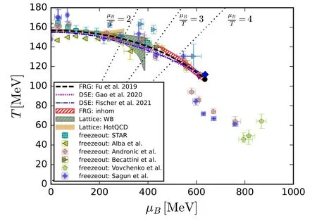
Figure 43.Phase diagram of Nf=2+1 flavor QCD in the plane of the temperature and the baryon chemical potential.The fRG results[18]are compared with those from Dyson–Schwinger equations[19,20],lattice QCD [8,12].The hatched red area denotes the region of inhomogeneous instability for the chiral condensate found in the calculations of fRG.Some freeze-out data are also shown in the phase diagram: [175](STAR),[228](Alba et al),[4](Andronic et al),[229](Becattini et al),[230](Vovchenko et al),and [231](Sagun et al).
4.6.1.Region of inhomogeneous instability at large baryon chemical potential.At large baryon chemical potentials,it is found within the fRG approach to QCD,that the mesonic wave function renormalization in equations (186) and (187)develops negative values at small momenta[18].As shown in figure 44 the mesonic wave function renormalization at vanishing external momenta Zφ,k=0(0) is depicted as a function of the temperature with several different values of μB.One can see a negative Zφ,k=0(0) begins to appear for a temperature region when μB≿420 MeV.The negative regime is clearly shown in the right plot ofbetween the two spikes,and it widens with the increase of the baryon chemical potential.From the two-point correlation functions of mesons,as shown in equations (186) and (187),the negative Zφ,k=0(0)implies that,for the dispersion relations of mesons,there is a minimum at a finite p2≠0.This nontrivial behavior that the minimum of dispersion is located at a finite momentum is indicative of an inhomogeneous instability,for instance,the formation of a spatially modulated chiral condensate.However,it should be reminded that a negative Zφ,k=0(0) is not bound to the formation of an inhomogeneous phase,it can also serve as a precursor for the inhomogeneous phase.See,e.g.[135,137,235–244]for more related discussions.Most notably,very recently consequence of the inhomogeneous instability indicated by the negative wave function renormalization on the phenomenology of heavy-ion collisions has been studied.It is found that this inhomogeneous instability would result in a moat regime in both the particle pTspectrum and the twoparticle correlation,where the peaks are located at nonzero momenta [243,244].The region of negative Zφ,k=0(0) is shown in figure 45 by the blue area,while the red hatched area shows where this region overlaps with a sizable chiral condensate.
Figure 44.Left panel:Mesonic wave function renormalization at vanishing external momenta Zφ,k=0(0)as a function of the temperature with several different values of the baryon chemical potential,obtained in the fRG approach to Nf=2+1 flavor QCD.Right panel:∣ ( 0)∣for the data in the left panel. The spikes are used to locate the region of negative Zφ,k=0(0). The plots are adopted from [18].
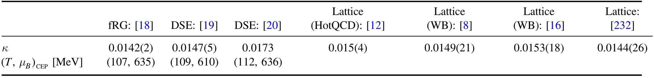
Table 2.Curvature к of the phase boundary(second line)and location of CEP(third line)for Nf=2+1 flavor QCD,obtained from different approaches.fRG:[18](Fu et al);DSE:[19](Gao et al),[20](Gunkel et al);Lattice QCD:[12](HotQCD),[8,16](WB),[232](Bonati et al).
4.7.Magnetic EoS
From equations (222),(224),and (225),it is convenient to define the corresponding susceptibilities for the light quark condensate,the renormalized light quark condensate,and the reduced condensate,i.e.
with (i)=(l),(l,R),(l,s) [62].Similar to the difference between the light quark condensate and the renormalized light quark condensate,the susceptibilities for them differ by the vacuum contribution.Among these three susceptibilities,the reduced susceptibility for the reduced condensate defined in fRG and lattice QCD,e.g.[13],matches better.
In figure 46 the susceptibility obtained from the reduced condensate as a function of the temperature for different pion masses in the fRG approach[62],is compared with the lattice results [13].One can see that the fRG results are in good agreement with the lattice ones for pion masses mπ≿100 MeV.There are some slight deviations from the two approaches for small pion masses.From the dependence of the reduced susceptibility on the temperature for a fixed pion mass in figure 46,one is able to define the pseudocriticalTcfRG≈142 MeV from the fRG approach [62],and temperature for the chiral crossover at such a value of pion mass,via the peak position of the curves,denoted by Tpc.
Figure 47 shows the dependence of the pseudocritical temperature on the pion mass,obtained both from the fRG approach and the lattice QCD.The values of pseudocritical temperature at finite pion masses are also extrapolated to the chiral limit,i.e.mπ→0,which leaves us with the critical temperature Tcin the chiral limit.One obtainsTclattice=MeV from the lattice QCD [13],that is,the critical temperature obtained in fRG is a bit larger than the lattice result.Recently,the critical temperature in the chiral limit from DSE is found to beTcDSE≈141 MeV [246].
From the general scaling hypothesis,see e.g.[66],in the critical regime the pseudocritical temperature scales with the pion mass as
where c is a non-universal coefficient,while the exponent p is related to the critical exponents β and δ through p=2/(βδ)[62].Inputting the values of β and δ for the 3-d O(4) universality class[196,247,248],one arrives at p ≈1.08.On the contrary,fitting the fRG data in figure 47 leads top≈[62].This discrepancy indicates that the pion masses under investigation in [62],i.e.mπ≿30 MeV are beyond the critical regime.In fact,the critical regime is found to be extremely small,mπ≾1 MeV,in fRG studies of LEFTs,and see,e.g.[98,151,186,198]for a more detailed discussion.
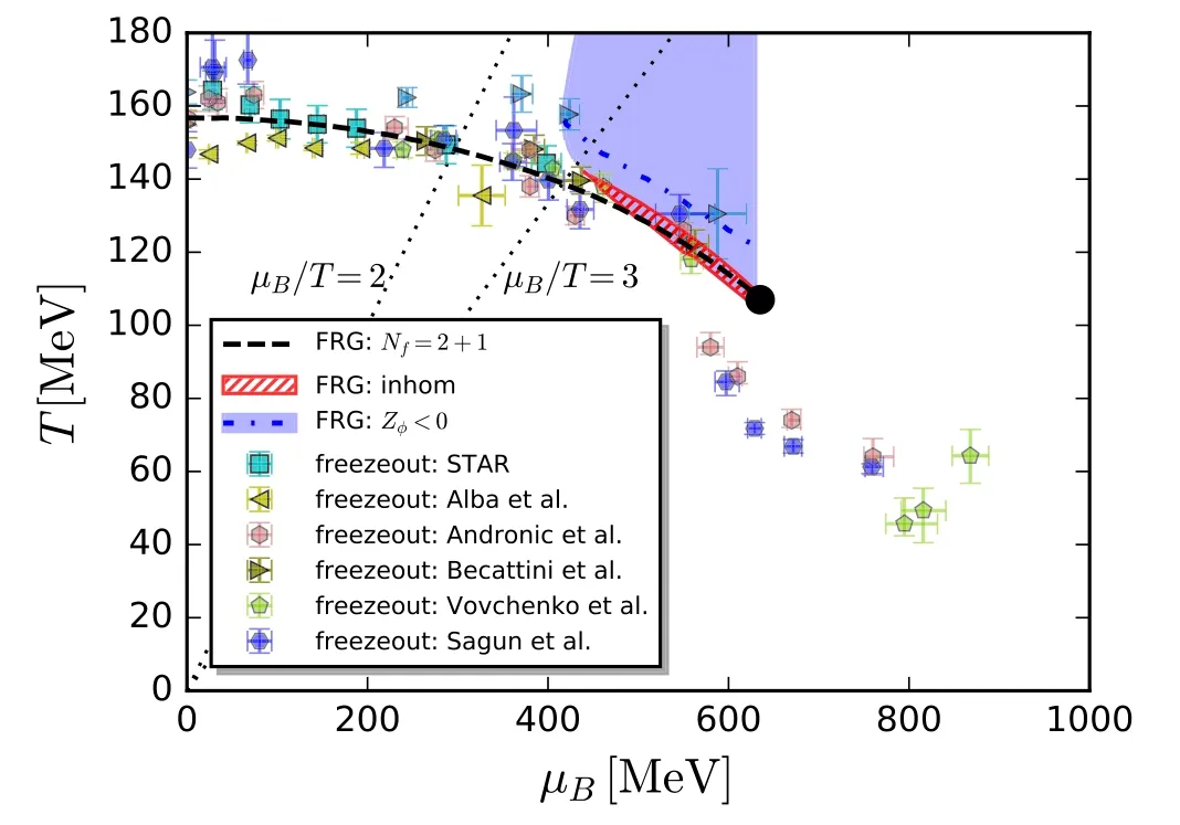
Figure 45.Phase diagram of Nf=2+1 flavor QCD obtained in the fRG approach to QCD in comparison to freeze-out data.See also the caption of figure 43.The blue area denotes the region of negative mesonic wave function renormalization at vanishing external momenta Zφ,k=0(0),which is an indicator of inhomogeneous instability.The red hatched area stands for the regime with negative Zφ,k=0(0) and also sizable chiral condensate.The plot is adapted from [18].
5.Real-time fRG
In this section,we would like to give a brief introduction to the real-time fRG,based on a combination of the fRG approach and the formalism of Schwinger–Keldysh path integral,where the flow equations are formulated on the closed time path.The Schwinger–Keldysh path integral is devised to study real-time quantum dynamics [249,250],which has been proved to be very powerful to cope with problems of both equilibrium and nonequilibrium many-body systems,see,e.g.[251–254]for relevant reviews.
Within the fRG approach on the closed time path,nonthermal fixed points of the O(N)scalar theory are investigated[255,256].The transition from unitary to dissipative dynamics is studied [257].Spectral functions in a scalar field theory with d=0+1 dimensions are computed within the real-time fRG approach [258].Moreover,it has also been employed to study the nonequilibrium transport,dynamical critical behavior,etc in open quantum systems[259,260],see also[55,254]for related reviews.Recently,the real-time fRG is compared with other real-time methods [261].
Furthermore,it should be mentioned that another conceptually new fRG with the Keldysh functional integral is put forward in [262–265],and the regulation of the RG scale there is replaced with that of the time,which is also called the temporal RG.Noteworthily,recently the Källén–Lehmann spectral representation of correlation functions has been used in the approach of DSE,to study the spectral functions in the φ4-theory and Yang–Mills theory [266–268].The spectral functions provide important information on the time-like properties of correlation functions,see,e.g.[269–272].Besides the real-time fRG,another commonly adopted approach is the analytically continued fRG,where the Euclidean flow equations are analytically continued into the Minkowski spacetime on the level of analytic expressions with some specific truncations,and see,e.g.[112,129,273–275]for more details.

Figure 46.Susceptibility for the reduced condensate obtained in the fRG approach to Nf=2+1 flavor QCD(fQCD)as a function of the temperature,in comparison to the lattice results in [13,245].The plot is adapted from [62].
In this section,we would like to discuss the fRG formulated on the Keldysh path at the example of the O(N)scalar theory [276].
5.1.fRG with the Keldysh functional integral
On the closed time path the classical action in equation(1)for a closed system reads
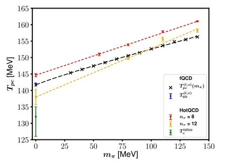
Figure 47.Pseudocritical temperature as a function of the pion mass obtained in fRG(fQCD)in comparison to the lattice results[13].The critical temperature in the chiral limit Tc has been obtained from an extrapolation of the pseudocritical temperature Tpc to mπ→0.The plot is adapted from [62].
It is more convenient to adopt the physical representation in terms of the ‘classical’ and ‘quantum’ variables,denoted by subscripts c and q,respectively,which are related to variables on the two-time branches by a Keldysh rotation,that is,

and

Then,equation (235) reads
The bilinear regulator term in equation (2) can be chosen as
Then the RG scale k-dependent generating function equation (1) with the Keldysh functional integral reads
The Schwinger functional in equation (14) reads

Combining the indices c,q and i for other degrees of freedom into one single label,say a,i.e.
One is able to simplify notations significantly,for instance,the regulator term in equation (239) now reading
with
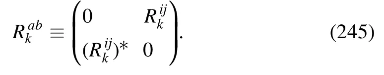
In the same way,the expectation value of the field reads
and the propagator is given by
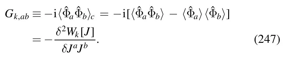
The effective action is obtained from the Schwinger functional upon a Legendre transformation,viz.,

Similar to equations (20) and (21),one has
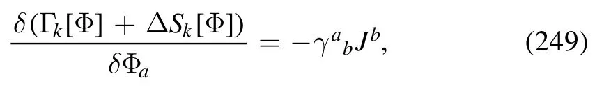
and

with
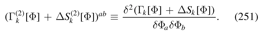
Then it is left to specify the flow equation of Schwinger functional with the Keldysh functional integral,which reads
where the RG time is denoted byτ≡ln(k、Λ),andRkTstands for the transpose of the regulator only in the c–q space as shown in equation (245).Finally,the flow equation of the effective action reads
5.2.Real-time O(N) scalar theory
The Keldysh effective action in equation (248) for the O(N)scalar theory reads
where the potential is given by

withρ±=Here φi,±and φi,c/q(i=0,1,…N-1)denote the fields of N components on the closed time branches or in the physical representation,respectively,and their relations are given in equation (236).Note that in equation (254) a local potential approximation with a kdependent wave function renormalization Zφ,khas been adopted,which is usually called the LPA’ approximation.
When the O(N) symmetry is broken into the O(N-1)one in the direction of component i=0,the expectation values of the fields read
Then,the sigma and pion fields are given by

and
The sigma and pion masses read
The regulator in equation (245) in the case of the O(N)scalar theory reads
with
where one has

with
Here,the 3d flat regulator is used.
The flow equation of effective action in equation (253)with the regulator in equation (261) can be reformulated as
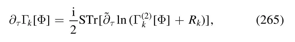
with
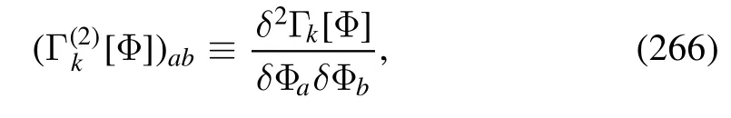
where the fluctuation matrix can be decomposed into a sum of the inverse propagatorPkand the interactionFkas shown in equation (58).In thermal equilibrium at a temperature T,the Pkmatrix reads
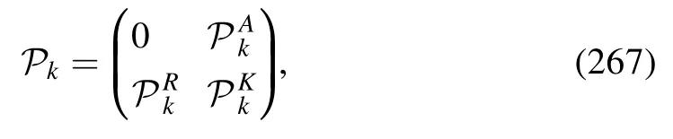
where the inverse retarded propagator is given by
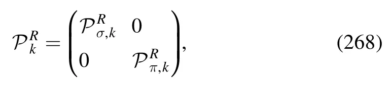
with
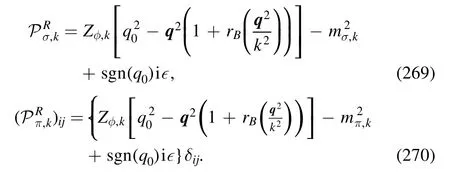
The inverse advanced propagator is related to the retarded one through a complex conjugate,to wit,
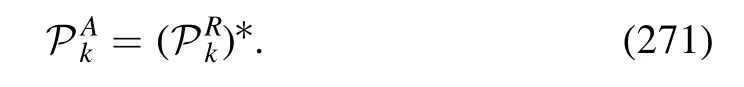
The qq component of the inverse propagator in equation (267),i.e.PkK,reads
with
Then,one can obtain the propagator matrix as follows
with the retarded and advanced propagator being

and the correlation function or Keldysh propagator being

Finally,one can verify the fluctuation-dissipation relation in thermal equilibrium,as follows
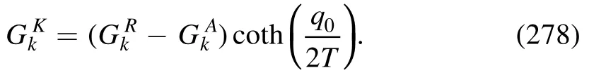
From equation (275) one arrives at the three different propagators which read
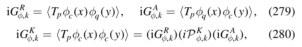
where Tpdenotes the time ordering from the positive to negative time branch in the Keldysh closed time path,and equation (280) follows directly from equation (277).The diagrammatic representation of these propagators is shown in figure 48.
Projecting the flow equation of the effective action in equation (265) onto a derivative with respect to the quantum sigma field σq,i.e.
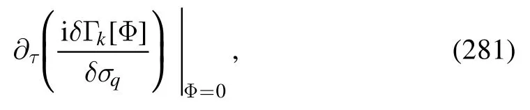
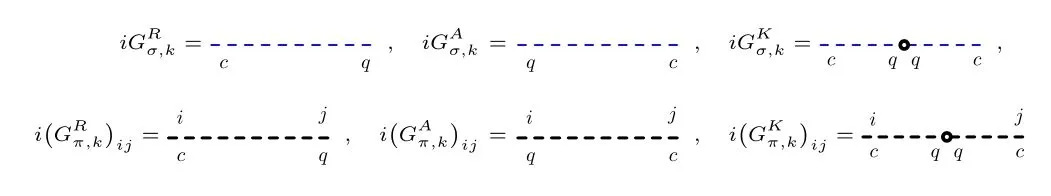
Figure 48.Diagrammatic representation of the three different propagators for the sigma and pion mesons.A line associated with two end points labelled with ‘c,q’ denotes the retarded propagator,while that with ‘q,c’ denotes the advanced propagator.A line with an empty circle inserted in the middle is used to denote the Keldysh propagator,which results from equation (277).The plot is adapted from [276].
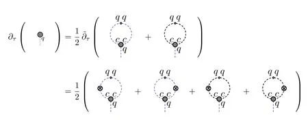
Figure 49.Diagrammatic representation of the flow equation of the effective potential in the real-time O(N) scalar theory.The vertices are denoted by gray blobs,and their legs are distinguished for the‘q’and ‘c’ fields.the crossed circles stand for the regulator insertion.The plot is adapted from [276].
with Φ=(σc,{πi,c},σq,{πi,q}),one is led to
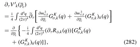
which is diagrammatically shown in figure 49.Integrating both sides of equation (282) over,one arrives at
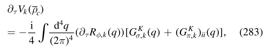
up to a term independent of.Inserting equations (269) and(270),one has
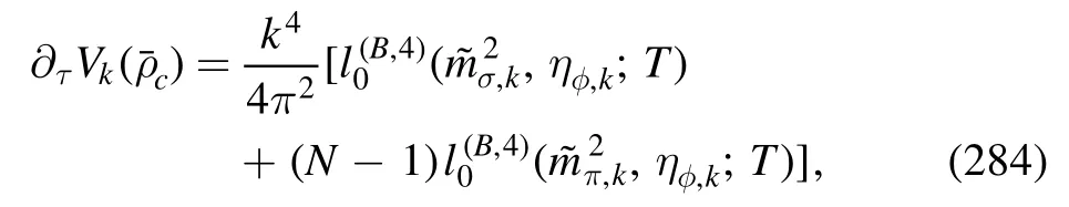
with the threshold function given by

and the renormalized dimensionless meson masses reading
where the bosonic distribution function reads
Note that equation (284) is just the flow equation of the effective potential in the LPA approximation obtained in the conventional Euclidean formalism of fRG.
5.3.Flows of the two-and four-point correlation functions
The 1PI n-point correlation function or vertex in the Euclidean field theory is given in equation(60),and the counterpart in the Keldysh field theory reads
Note that a label‘c’or‘q’is associated with an external leg of the vertex to distinguish the classical or quantum field,as shown in figure 49.In the following,we consider the symmetric phase with=0 in equation (256).In this case,the pion and sigma fields are degenerate,and they are collectively denoted by φi(i=0,1,…N-1).The diagrammatic representation of the four-point vertexreads
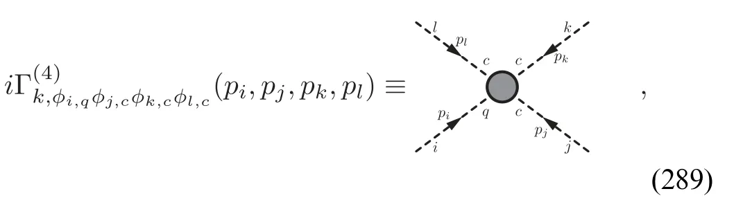
whose flow equation is given in figure 50.According to the generic interchange symmetry of the external legs,the fourpoint vertex can be parameterized as
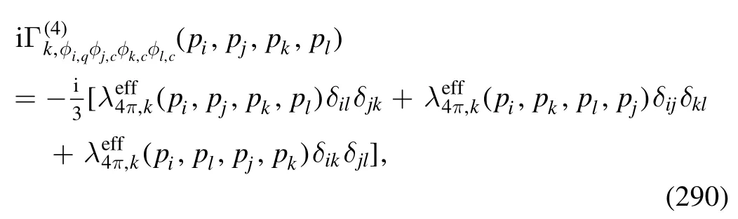
where an effective four-point couplingis introduced.In the following,one adopts the truncation that the momentum dependence of the four-point vertex on the r.h.s.of the flow equation in figure 50 is neglected,and the four-point vertex there is identified as
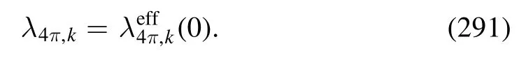
Then,from the flow of the four-point vertex in figure 50,one arrives at
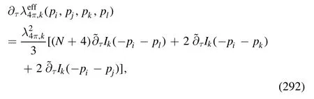
with
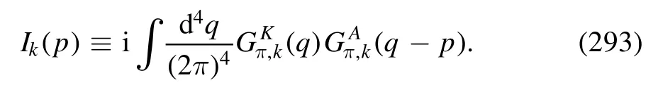
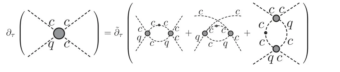
Figure 50.Diagrammatic representation of the flow equation of the four-point vertex in the symmetric phase.The plot is adapted from[276].
Note that the wave function renormalization Zφ,k=1 is
adopted to simplify the calculation of(p)in equation (292).The explicit expression of Ik(p) can be found in [276].
With the four-point vertex in equation (290) one is able to obtain the self-energy as follows
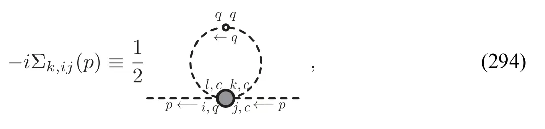
which reads
Here,the functionis given by
with θ being the angle between the two momenta p and q.The inverse retarded propagator,i.e.the two-point correlation function with one q field and one c field,is given by
and its flow equation reads
Substituting the Keldysh propagator in equation (277),one arrives at
The first part of the r.h.s.of equation (299) reads
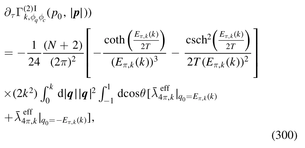
and the second part is given by
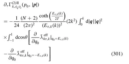

with wheremπ2,kcan be extracted from the two-point correlation function at vanishing momentum,viz.,
Note that the second part in equation(301)is negligible if the momentum dependence of the vertex is mild.
5.4.Spectral functions and dynamical critical exponent
The retarded propagator in the Källén–Lehmann spectral representation is related to the spectral function ρ via a relation as follows

Thus,the spectral function is proportional to the imaginary part of the retarded propagator,i.e.

Notice that here the IR limit k→0 is tacitly assumed.The retarded propagator is just the inverse of the two-point correlation function,to wit,

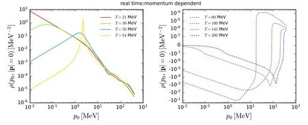
Figure 51.Spectral function ρ(p0,∣p∣=0)as a function of p0 with several small(left panel,close to the critical temperature Tc=20.4 MeV)and large (right panel) values of temperature obtained in the real-time O(4) scalar theory within the fRG approach.The plots are adapted from [276].
Consequently,the spectral function can be expressed in terms of the real and imaginary parts of the two-point correlation function,that is,
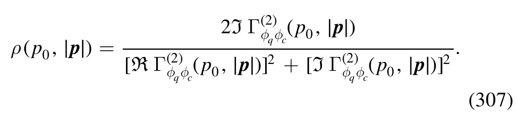
Evidently,one has
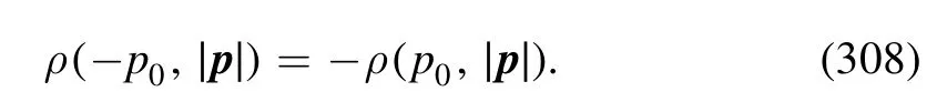
In figure 51,the spectral functionρ(p0,∣p∣=0)is shown as a function of p0with different values of the temperature.In the left panel,the temperatures are above but close to the critical temperature Tc=20.4 MeV for the phase transition,where the symmetry is broken from O(N) to O(N-1) when T<Tc,while in the right panel,the temperatures are far larger than Tc.One can see that when temperature is large,one has a negative spectral function in the regime of small p0,and there is a minus peak structure around the pole mass.It is found that the negative spectral function results from the contributions of the Landau damping,and see[276]for a more detailed discussion.Nonetheless,when the temperature is decreased below about 60 MeV,the Landau damping is dominated by the process of creation and annihilation of particles,and the spectral function is positive.Moreover,when the temperature is closer and closer to the critical temperature,the peak structure on the spectral function becomes wider and wider,and finally disappears at the critical temperature.The 3D plots of the spectral function as a function of p0and∣∣pare shown in figure 52 with two different values of the temperature.
We proceed to the discussion of the dynamical critical exponent,and begin with the kinetic coefficient Γ(∣p∣) that is defined as
where the parity properties of the real and imaginary parts of the two-point correlation function have been used,i.e.
The relaxation rate,or dissipative characteristic frequency,is given by
When the momentum is larger than the correlation length∣p∣ >ξ-1,withξ~mφ-1,the relaxation rate scales as

through which one can extract the dynamical critical exponent z [277].From figure 53 the value of the dynamical critical exponent in the real-time 3d O(4) scalar theory is extracted,and one arrives at z=2.02284(6),where the numerical error is shown in the bracket.
According to the standard classification for universalities of the critical dynamics [277],it is argued that the critical dynamics of the relativistic O(4) scalar theory belongs to the universality of Model G[278],see also[279],which leaves us with z=3/2 in three dimensions.The dynamic critical exponent for the O(4) model is also calculated in real-time classical-statistical lattice simulations,and it is found that z is in favor of 2,but there is still a sizable numerical error[279].The dynamic critical exponent in a relativistic O(N) vector model is also found to be close to 2[257].A similar result is found in a O(3) model in [280].Moreover,z=1.92(11) is found for Model A in three spatial dimensions from real-time classical-statistical lattice simulations [281].In short,the dynamic critical exponent is far from clear and conclusive in comparison to the static critical exponent,and more studies of the critical dynamics from different approaches,including the real-time fRG,are necessary and desirable in the future.
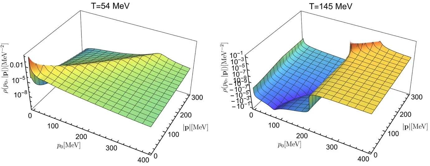
Figure 52.3D plots of the spectral function as a function of p0 and∣p∣at temperature T=54 MeV (left panel) and 145 MeV (right panel),obtained in the real-time O(4) scalar theory within the fRG approach.The plots are adapted from [276].

Figure 53.Double logarithm plot of the relaxation rate ω(∣p∣) in equation(313)as a function of the spatial momentum with p0=0 at the critical temperature Tc=20.4 MeV,obtained in the real-time 3d O(4) scalar theory within the fRG approach.The plot is adapted from [276].
6.Conclusions
In this paper,we present an overview on recent progress in studies of QCD at finite temperature and densities within the fRG approach.After a brief introduction of the formalism,the fRG approach is applied in low energy effective field theories 450 MeV ≾μBCEP≾650 MeV.Moreover,a region of inhoand the first-principle QCD.The mechanism of quark mass production and natural emergence of bound states is well illustrated within the fRG approach,and a set of self-consistent flow equations of different correlation functions provide the necessary resummations,and plays the same role as the quark gap equation and Bethe–Salpeter equation of bound states.
We present results for the QCD phase structure and the location of the CEP,the QCD EoS,the magnetic EoS,baryon number fluctuations confronted with recent experimental measurements,various critical exponents,etc.It is found that the non-monotonic dependence of the kurtosis of the net-baryon or net-proton (proxy for net-baryon in experiments) number distributions could arise from the increasingly sharp crossover with the decrease of the beam collision energy,which in turn indicates that the non-monotonicity observed in experiments is highly non-trivial.Furthermore,recent estimates of the location of the CEP from first-principle QCD calculations within fRG and DSEs,which pass through lattice benchmark tests at small baryon chemical potentials,converge in a rather small region at baryon chemical potentials of about 600 MeV.But it should be reminded that errors of functional approaches increase significantly in the regime of μB/T ≿4,and thus one arrives at a more reasonable estimation for the location of CEP as mogeneous instability indicated by a negative wave function renormalization is found with μB≿420 MeV,and its consequence on the phenomenology of heavy-ion collisions has been investigated very recently [243,244].It is found that this inhomogeneous instability would result in a moat regime in both the particle pTspectrum and the two-particle correlation.By investigating the critical behavior and extracting critical exponents in the vicinity of the CEP,it is found that the size of the critical region is extremely small,quite smaller than~1 MeV.
In this review,we also discuss the real-time fRG,in which the flow equations are formulated on the Schwinger–Keldysh closed time path.By organizing the effective action and the flow equations in terms of the‘classical’and‘quantum’fields,one is able to give a concise diagrammatic representation for the flow equations of propagators and vertices in the real-time fRG.The spectral functions of the O(N)scalar theory in the critical regime in the proximity of the critical temperature are obtained.The dynamical critical exponent in the O(4) scalar theory in 3+1 dimensions is found to be z ≃2.023.
Acknowledgments
I would like to thank Heng-Tong Ding,Xiaofeng Luo,Jan M Pawlowski,Bernd-Jochen Schaefer,Yue-Liang Wu for reading this manuscript and providing helpful comments.I thank Jens Braun,Yong-rui Chen,Chuang Huang,Zi-Wei Lin,Yu-xin Liu,Xiaofeng Luo,Guo-Liang Ma,Jan M.Pawlowski,Fabian Rennecke,Bernd-Jochen Schaefer,Yangyang Tan,Rui Wen,Yue-Liang Wu,Shi Yin for collaborating on related subjects.I am also grateful to Jens Braun,Yong-rui Chen,Heng-Tong Ding,Fei Gao,De-fu Hou,Chuang Huang,Mei Huang,Zi-Wei Lin,Yu-xin Liu,Xiaofeng Luo,Guo-Liang Ma,Jan M.Pawlowski,Fabian Rennecke,Bernd-Jochen Schaefer,Huichao Song,Yang-yang Tan,Rui Wen,Nicolas Wink,Yue-Liang Wu,Shi Yin,Yu Zhang,Peng-fei Zhuang for discussions on related subjects.I am very grateful to the authors of[159]for providing me with the unpublished results in figure 11.Moreover,I also would like to thank the members of the fQCD collaboration [282]for their discussions and collaborations.This work is supported by the National Natural Science Foundation of China under Grant No.12175030.
Appendix A.Flow equations of the gluon and ghost self-energies in Yang–Mills theory at finite
temperature
A.1.Feynman rules
First of all,we present the Feynman rules for relevant propagators and vertices at finite temperatures and densities.
A.1.1.Gluon propagator
The kinetic term for the gluon field in equation (48) in momentum space is given by
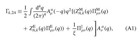
where the magnetic projection operator reads
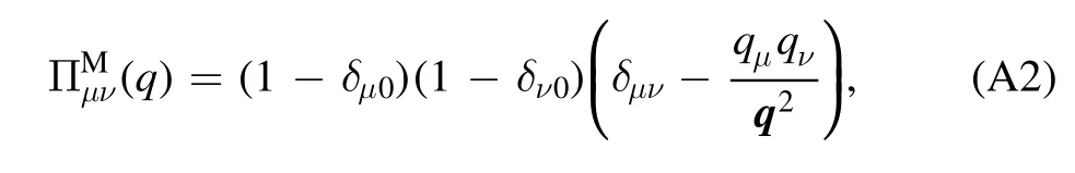
and the electric projection operator
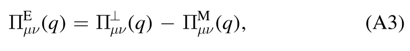
with the transverse and longitudinal tensors given by
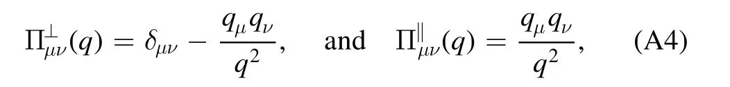
respectively.Note that in equation (A1) different magnetic and electric gluonic dressing functions,i.e.ZAM,k(q) ≠ZAE,k(q),are assumed at finite temperature.Differentiating equation (A1) w.r.t.the gluon field twice,one obtains
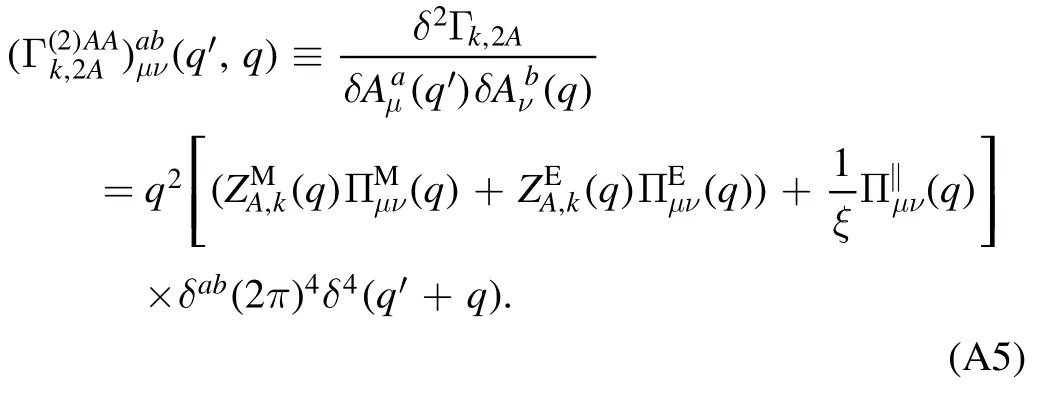
Moreover,the regulator for the gluon reads
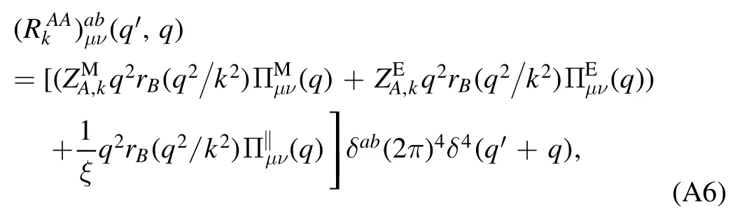
whereandare independent of momentum q by contrast to those in equation (A5).The threshold function rB(x) can be chosen to be that in equation (10) or (12).Therefore,the gluon propagator is readily obtained from equation (21),as follows

with

where one has
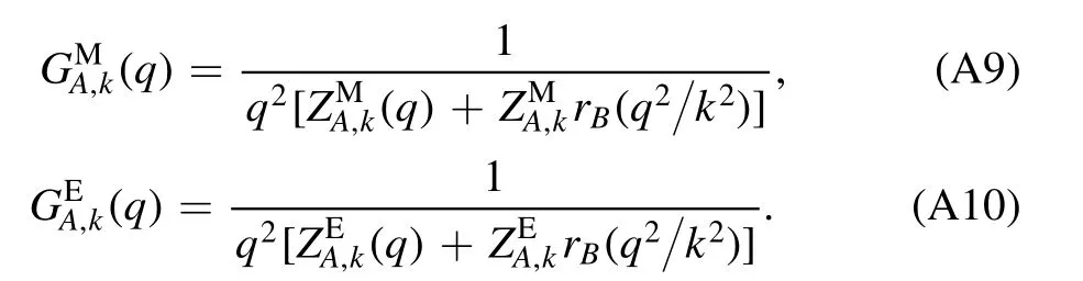
Here the gauge parameter is chosen to be ξ=0.
A.1.2.Ghost propagator
In the same way,the kinetic term for the ghost field in equation (48) reads
where we have used the convention of Fourier transformation for the Grassmann fields as follows
Then,it follows that
and
Note that,for a Grassmann field,the relation such as

always holds.The regulator for the ghost field reads
whose inverse matrix is just the ghost propagator which is given by
with
Recovering the indices,one obtains the ghost propagator as follows
with
A.1.3.Quark propagator
The kinetic term for the quark field in equation (48) reads
It follows that
and
The regulator reads
TheP matrix for the quark field reads
and the relevant propagator is given by
with
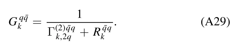
Displaying the momentum explicitly,one arrives at the quark propagator as follows
with
A.1.4.Ghost-gluon vertex
First of all,we consider the case in a vacuum.The action relevant to the ghost-gluon interaction in equation (48) reads
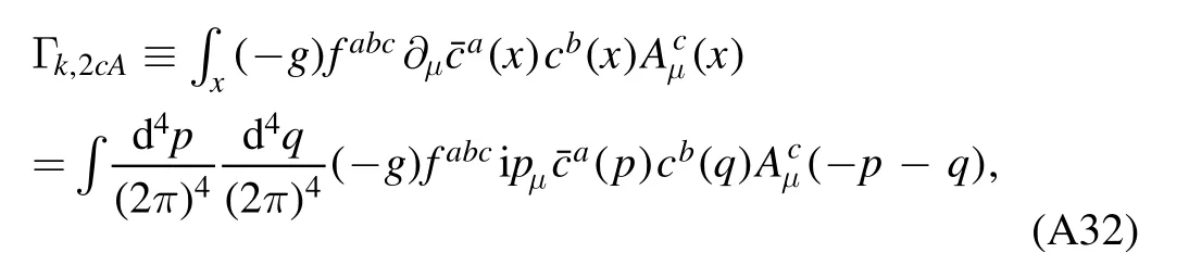
which yields
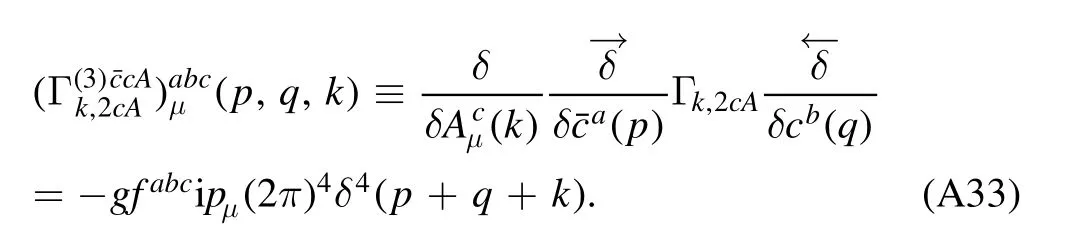
Thus,the Feynman rule for the ghost-gluon vertex in the vacuum is given as follows
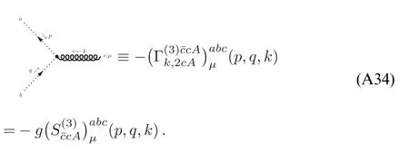
with the classical tensor of the ghost-gluon vertex defined by
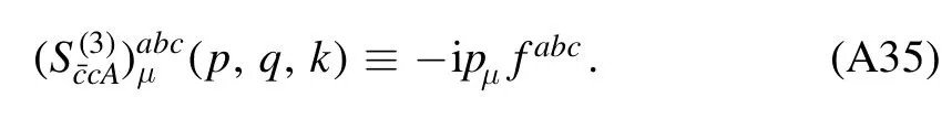
At finite temperature,the external leg of gluon would be split into the magnetic and electric sectors,and thus the general form for the ghost-gluon vertex at finite temperature reads
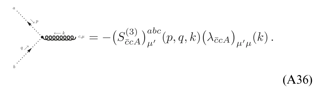
with
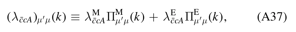
A.1.5.Three-and four-gluon vertices
From the effective action in equation (48),one is able to obtain the three-gluon vertex in the vacuum,as follows
with the classical three-gluon tensor
In the same way,the four-gluon vertex reads
with the classical four-gluon tensor
Similar to the case of ghost-gluon vertex,each external leg of the three-and four-gluon vertices should be split into a sum of the magnetic and electric components at finite temperature,and see,e.g.[57]for more details.Consequently,the three-gluon vertex at finite temperature reads
with
the projector with one electric gluon and two magnetic gluons
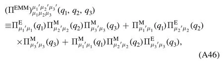
the projector with two electric gluons and one magnetic gluon
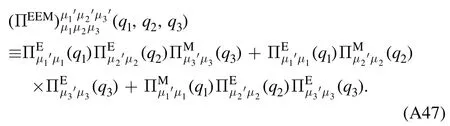
The four-gluon vertex at finite temperature reads
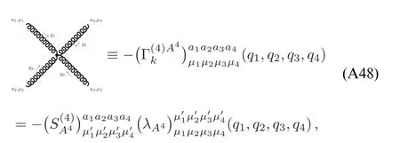
with
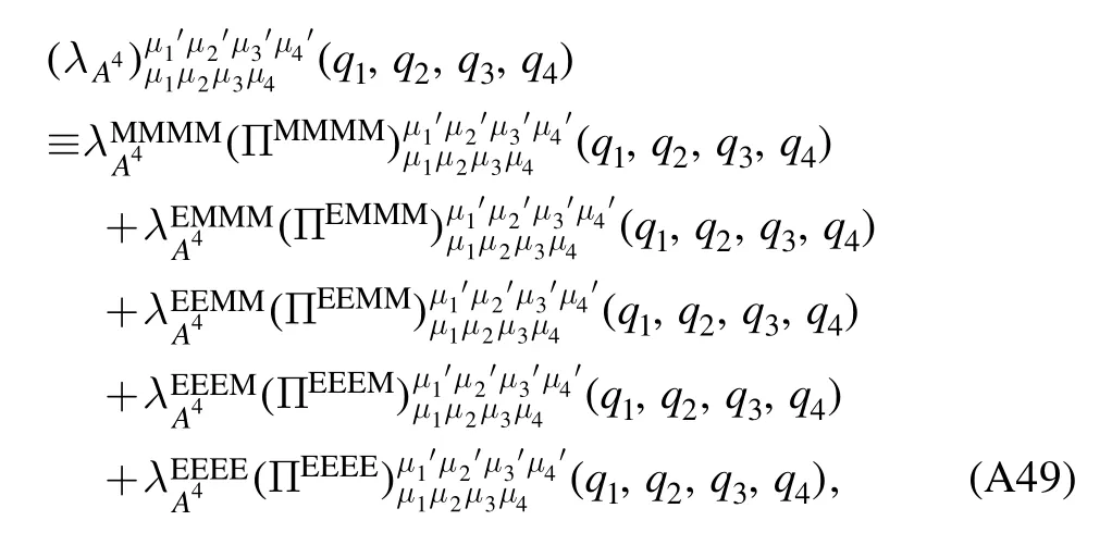
and
the projector with one electric gluon and three magnetic gluons
the projector with three electric gluon and one magnetic gluons

the projector with two electric gluons and two magnetic gluons
A.2.Gluon self-energy
With the Feynman rules discussed in section A.1,it is straightforward to write down expressions for the loop diagrams of the gluon self-energy as shown on the r.h.s.of flow equation in figure 3.The first gluon loop reads
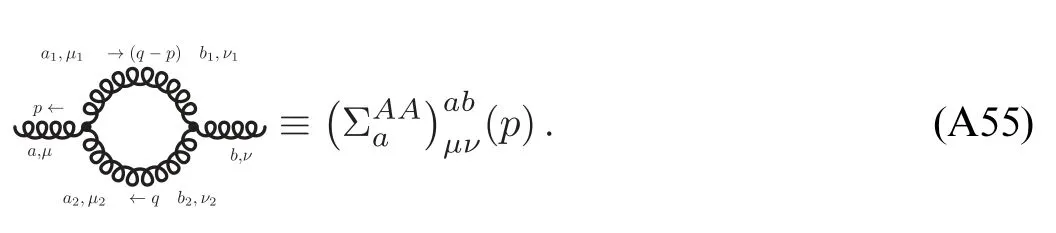
with
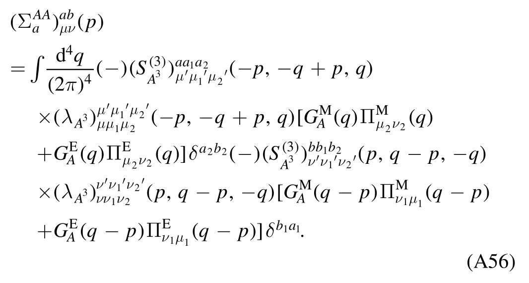
Projecting equation(A56)onto the magnetic component,one arrives at
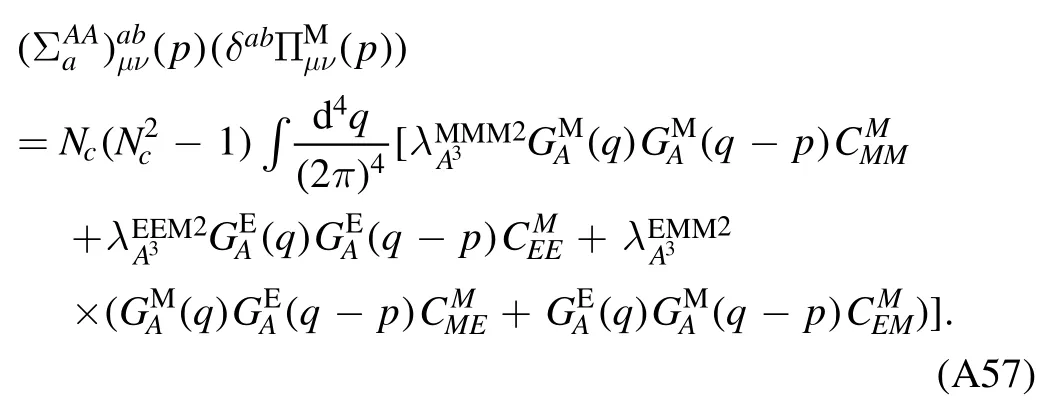
Here we have defined several coefficients,which reads
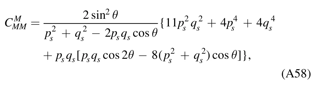
where the two 4-momenta are p=(p0,p)and q=(q0,q),withps= ∣p∣,qs=|q| and cosθ=In the same way,
we have
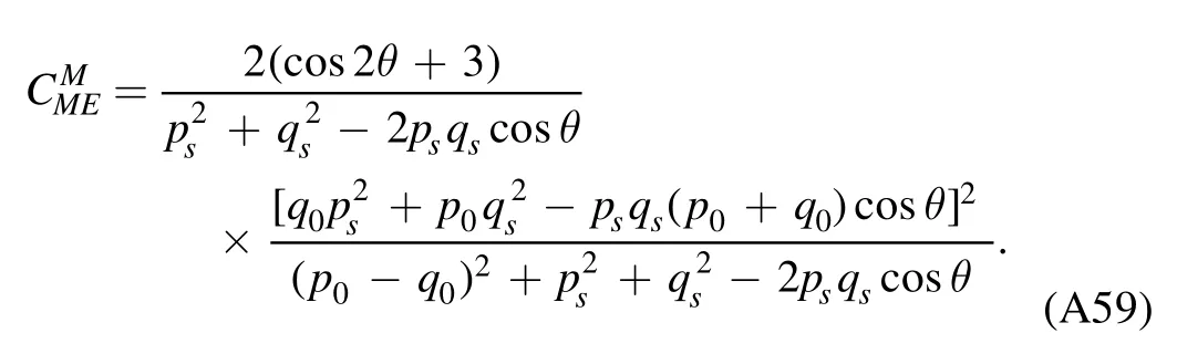
The coefficient CMEMcould be deduced from CMMEthrough the replacement as follows
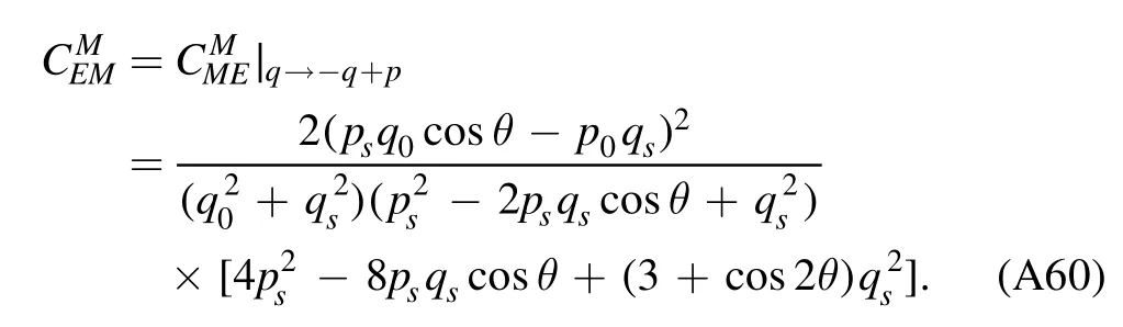
Finally,the last one is given by
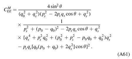
Projection of equation(A56)onto the electric component yields
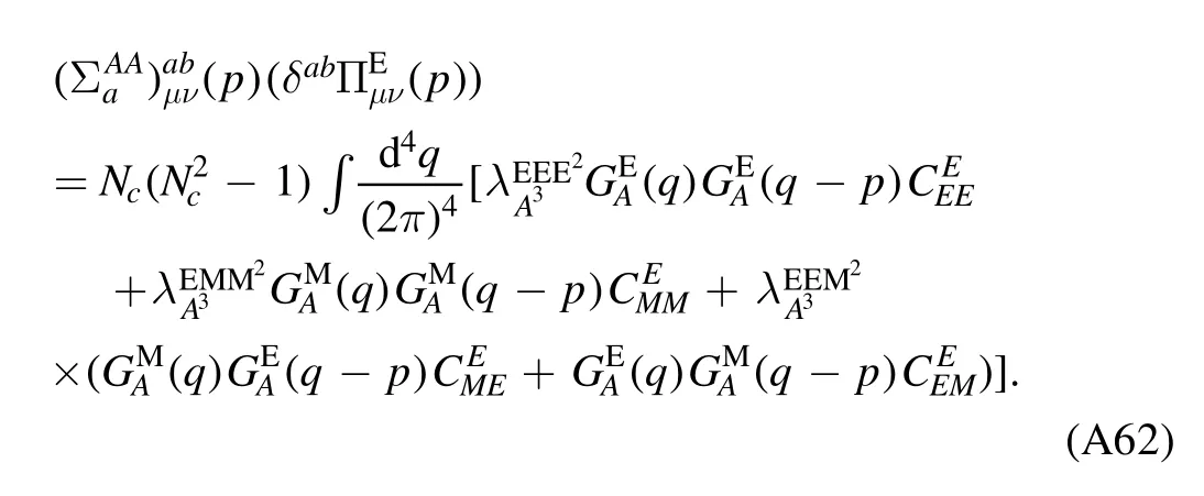
There are four coefficients as well,and their explicit expressions are given as follows,
coefficient CEME
coefficient CEEM
and coefficient CEMM
The ghost loop of the gluon self-energy,i.e.the second diagram on the r.h.s.of flow equation in figure 3,reads
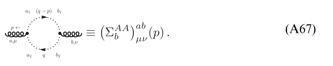
with

Projecting equation(A68)onto the magnetic component leads us to
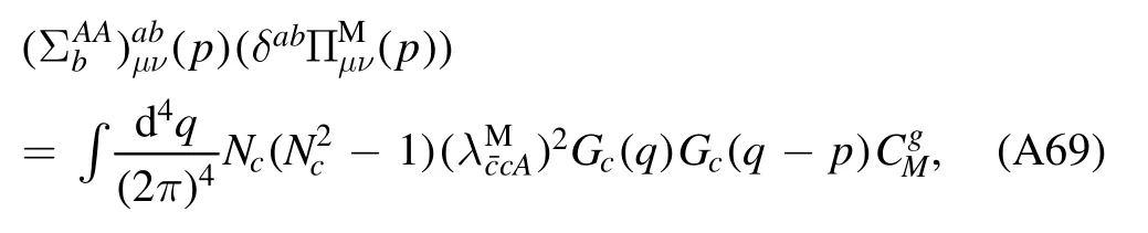
with
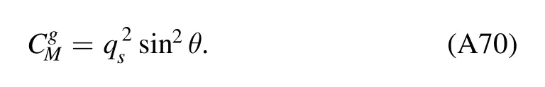
And the electric component is given by
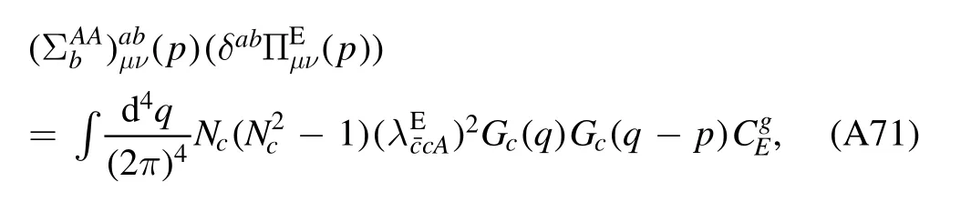
with
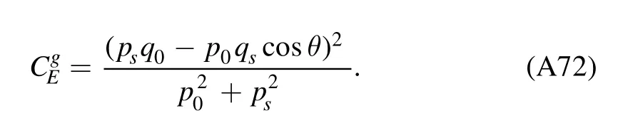
The tadpole diagram of the gluon self-energy due to the four-gluon vertex,i.e.the third diagram on the r.h.s.of flow equation in figure 3,reads
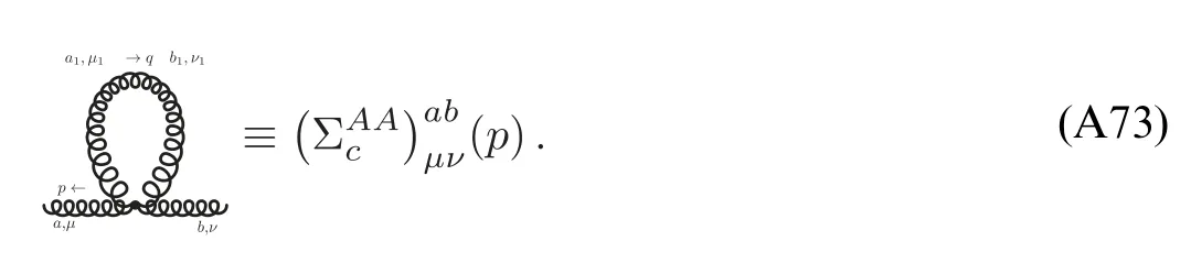
with
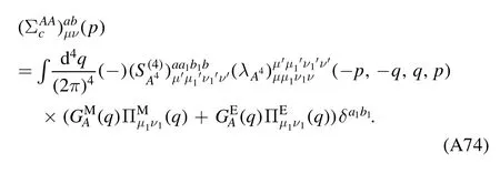
Projecting equation (A74) onto the magnetic component leaves us with
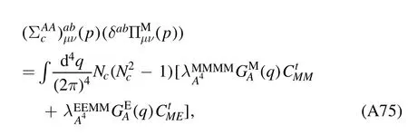
with
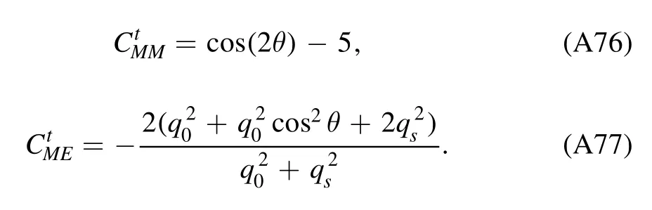
The electric component reads
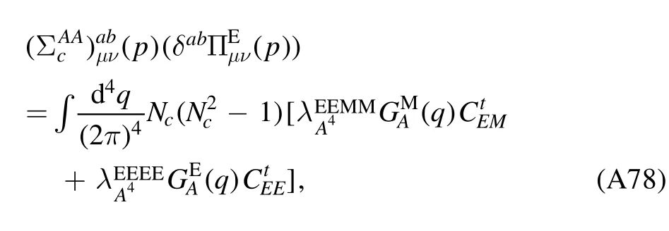
with
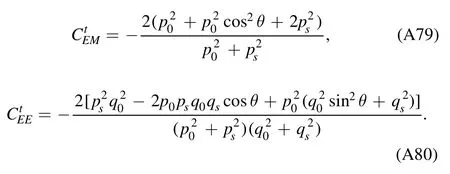
Substituting equations (A57),(A62),(A69),(A71),(A75),(A78) into the flow equation in figure 3,one obtains the flow equation of the magnetic gluon dressing function
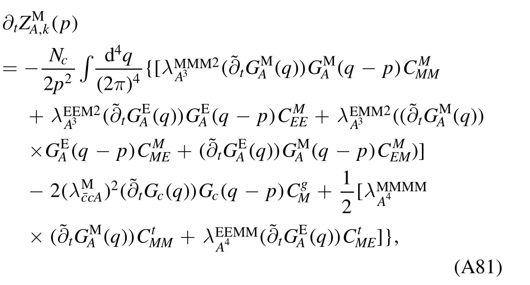
and the flow equation of the electric gluon dressing function
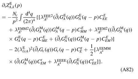
A.3.Ghost self-energy
The flow equation of the ghost self-energy in Yang–Mills theory is depicted in figure 54.The one-loop diagram on the r.h.s.reads
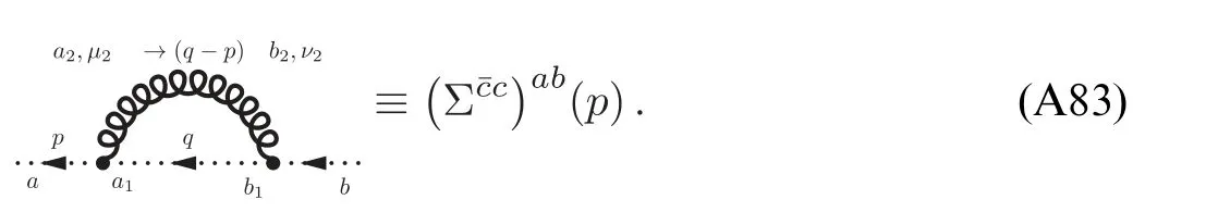
with
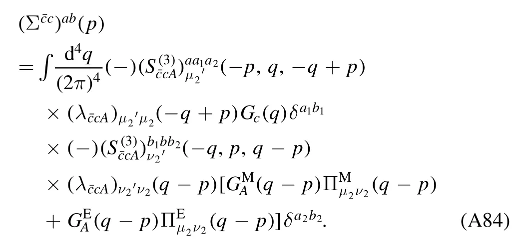
Tracing the color indices,one arrives at
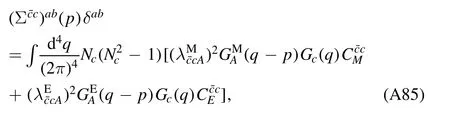
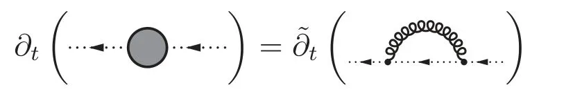
Figure 54.Diagrammatic representation of the flow equation for the ghost self-energy in Yang–Mills theory.
with
In the following,we also need the expression in equation (A85) with the replacement of the internal momentum q→-q+p,which reads
with
Finally,inserting equations (A85) and (A88) into the flow equation in figure 54,one is led to the flow equation of the ghost dressing function,as follows
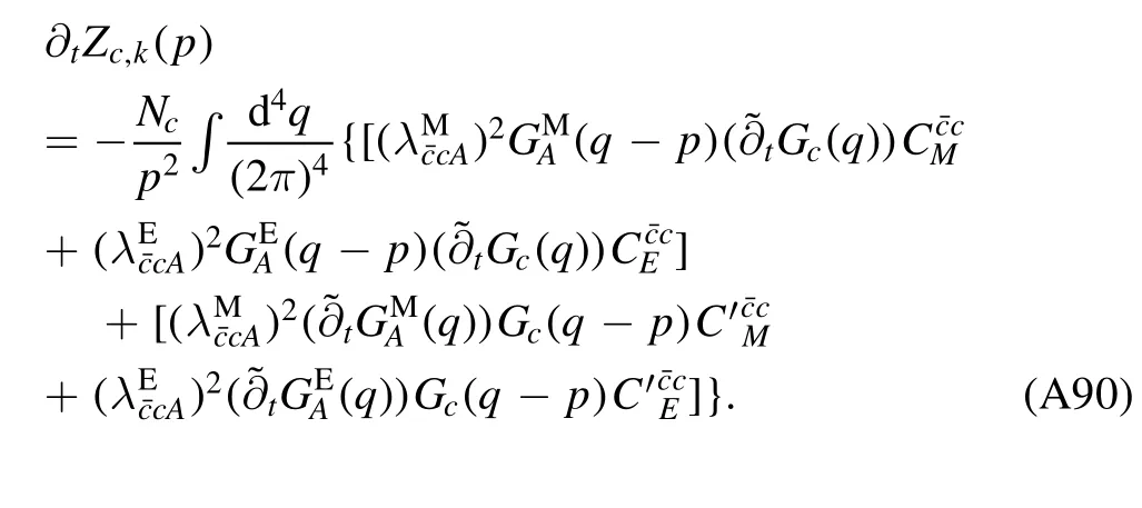
Appendix B.Fierz-complete basis of four-quark interactions of Nf=2 flavors
Here we list the Fierz-complete basis of four-quark interactions of Nf=2 flavors equation(82),see also e.g.[58,61,92].The ten different channels can be classified into four different subsets according to their invariance or not,under the global transformations of the groups SUV(Nf),UV(1),SUA(Nf),and UA(1).Of the ten channels,several are invariant under all the transformations mentioned above,which read
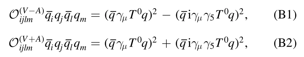

where generators of the flavor SU(Nf) group and the color SU(Nc)group are denoted by Ta's and ta's,respectively,and summation for the indices is assumed.Furthermore,one hasAnother two channels,given by
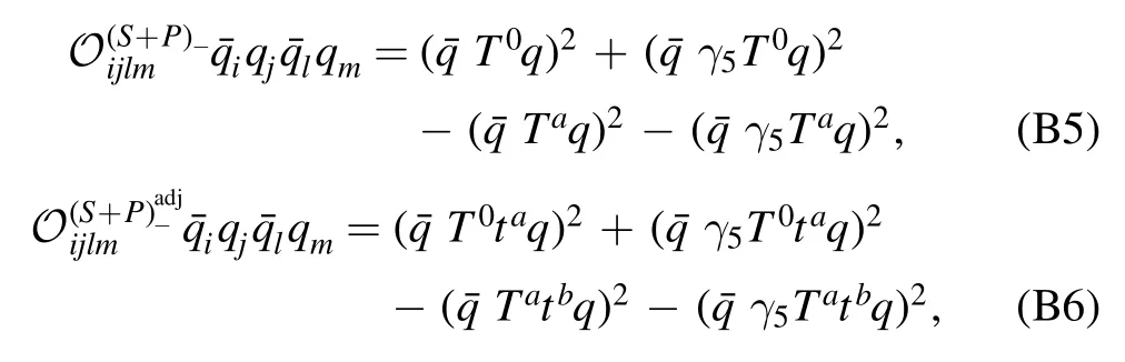
break the symmetry of UA(1) while preserving SUV(Nf)⊗UV(1)⊗SUA(Nf).The two channels that read
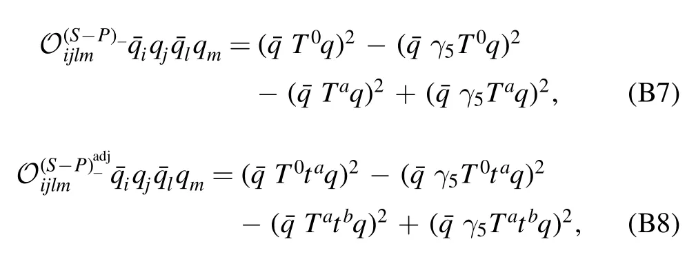
break SUA(Nf) while preserving SUV(Nf)⊗UV(1)⊗UA(1).The last two independent channels,viz.,
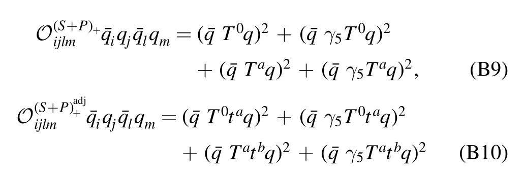
break both UA(1) and SUA(Nf),while preserving SUV(Nf)⊗UV(1).
Moreover,it is also useful to combine linearly several different channels of the four-quark couplings to form new independent elements of basis.For instance,the four scalarpseudoscalar channels as follows are obtained from linear combinations of O(S-P)+in equation (B3),O(S+P)-in equation (B5),O(S-P)-in equation (B7),and O(S+P)+in equation (B9).
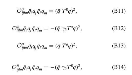
Appendix C.Some flow functions
In this appendix,we present explicit expressions for some flow equations.The threshold functions involved in this appendix can be found in,e.g.[18,148].
The anomalous dimension of quarks ηq,kin equation (185) reads

with Nf=2 and Nc=3.The anomalous dimension of mesons at p=0 in equation (191) reads
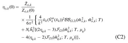
and that at p0=0 and p2=k2in equation (189) reads
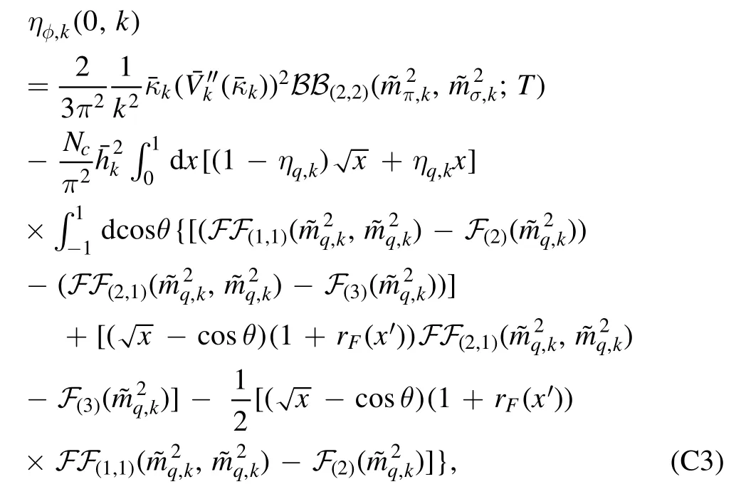
The contribution to the gluon anomalous dimension from the quark loop reads
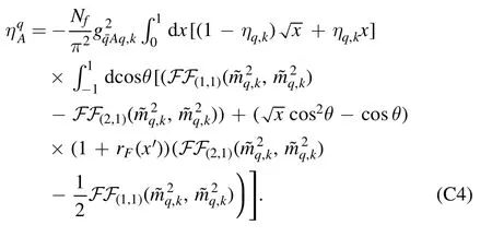
As same as in equation (C3),the external momentum in equation (C4) is chosen to be∣p∣=k.The in-medium contribution from the light quarks,included in equation(194),is given by
with=,Nf=2 and the light-quark–gluon coupling,in equation(C4).For the strange quark,since the vacuum contribution is also presented in equation (195),one needs
which is obtained from equation (C4) with=,Nf=1 and the strange-quark–gluon coupling.
The second term on the r.h.s.of equation (194),,denotes the contribution to the gluon anomalous dimension from the thermal part of the glue sector,which is taken into account through the thermal screening mass of gluons.The modified gluon anomalous dimension reads
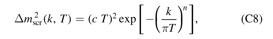
where c=2 is adopted for Nf=2+1,which is consistent with the result in[57].Furthermore,n=2 is chosen in equation(C8).
The flow of the quark–gluon couplings in equations (205)and (206) are given by
and
Here for the light-quark–gluon coupling in equation (205) we use the light quark mass and Nf=2,and for the strange-quark–gluon coupling in equation(206)we use the strange quark mass and Nf=1.
The flow of the four-quark coupling in the σ–π channel from two gluon exchanges in equation (214),as diagrammatically shown in the first line of figure 34,reads
The contributions to the flow of four-quark coupling from two meson exchanges,as shown in the second line of figure 34,reads

The flow of the Yukawa coupling in equation(219)reads
ORCID iDs
杂志排行
Communications in Theoretical Physics的其它文章
- Preface
- Phase behaviors of ionic liquids attributed to the dual ionic and organic nature
- Chaotic shadows of black holes: a short review
- The Gamow shell model with realistic interactions: a theoretical framework for ab initio nuclear structure at drip-lines
- Effects of the tensor force on low-energy heavy-ion fusion reactions: a mini review
- Relativistic Hartree–Fock model and its recent progress on the description of nuclear structure*