Koopman analysis of nonlinear systems with a neural network representation
2022-10-22ChufanLiandYuehengLan
Chufan Li and Yueheng Lan,2
1 School of Science,Beijing University of Posts and Telecommunications,Beijing 100876,China
2 State Key Lab of Information Photonics and Optical Communications,Beijing University of Posts and Telecommunications,Beijing 100876,China
Abstract The observation and study of nonlinear dynamical systems has been gaining popularity over years in different fields.The intrinsic complexity of their dynamics defies many existing tools based on individual orbits,while the Koopman operator governs evolution of functions defined in phase space and is thus focused on ensembles of orbits,which provides an alternative approach to investigate global features of system dynamics prescribed by spectral properties of the operator.However,it is difficult to identify and represent the most relevant eigenfunctions in practice.Here,combined with the Koopman analysis,a neural network is designed to achieve the reconstruction and evolution of complex dynamical systems.By invoking the error minimization,a fundamental set of Koopman eigenfunctions are derived,which may reproduce the input dynamics through a nonlinear transformation provided by the neural network.The corresponding eigenvalues are also directly extracted by the specific evolutionary structure built in.
Keywords: deep learning,autoencoder,Koopman operator,Van der Pol equation,coupled oscillator
1.Introduction
Equilibrium statistical physics is well established and great efforts have been made to extend the theory to treat nonequilibrium systems.Nevertheless,success is limited due to the lack of detailed balance and the intrinsic complexity of system dynamics.It has been realized that nonlinearity is a hallmark of a system with complex dynamics,giving rise to rich diversity of system behaviour across physical,biological,social and engineering sciences [1,2],which are hard to characterize and reliably analyze [3–8].
Much progress has been made in the analysis of lowdimensional nonlinear systems and various techniques are developed to probe their phase spaces.Most often,these approaches are focused on the study of individual orbits,especially those that organize system dynamics.Nevertheless,in systems with higher dimensions,especially in complex systems,typical orbits could become very unstable and extremely intertwined,being hard to characterize.In this case,a coarse-grained description may better suit our needs,which should be able to feature the global dynamics by ignoring irrelevant details,much similar to what has been done in statistical mechanics.Fortunately,the Koopman operator provides such a tool that drives the evolution of functions(also called observables)defined in a phase space[9]and thus shifts the focus to the ensemble of trajectories.In the early days,theoretical aspects of this operator were discussed in statistical or mechanical systems [10–12].In recent years,a surge of Koopman analysis and its applications pervade diverse fields,such as power systems [13–16],building energy efficiency models [17],fluid systems [18–21],chemistry [22],robotics [23–25]and biology [26–28].
Koopman operator is a linear operator and thus many well-developed linear analysis tools could be adapted to its computation.For example,the evolution of a dynamical system is described by its eigenvalues and eigenfunctions,against which scalar or vectorial observables could be expanded.The expanding coefficients are called Koopman modes [13].An algorithm called dynamic mode decomposition(DMD)was proposed by Schmid[29]based on the wellknown singular value decomposition (SVD) to calculate Koopman modes.The idea of decomposition was further pursued with variants featuring different choices of Koopman invariant subspaces or alternative ways to compute its spectral properties [20,30,31].One advantage of the Koopman analysis is that it could be directly used to treat data acquired from simulation or measurements without knowing the underlying equations of motion,which could be hard to write down,especially in complex systems.That is probably why it has been widely applied in various systems.The early wave of this development in both theory and applications was reviewed by Budisic et al [32].
As the Koopman operator lives in a functional space,often a large family of eigenvalues and eigenfunctions are obtained in a matrix approximation of the operator.But we are mostly interested in those that capture the main features of the system dynamics,characterized by the atomic part of the spectrum.Therefore,an effective application of the Koopman analysis usually involves a great reduction of dimension which is similar to what has been achieved in deep neural networks (DNNs) [33].The problem is how to find this reduction and how to represent the reduced function space.On the other hand,the universal approximation theorem of the neural network states that if a network contains enough neurons,theoretically it can approximate any continuous function [34–36].Therefore,the DNN is a natural candidate to enable a scalable and data-driven architecture for the discovery and representation of the principal Koopman modes[37–40].Takeishi et al[41]introduced a set of functions with a neural network by minimizing the residual sum of squares.However,one possible drawback of such an implementation stems from possible trapping in local optima of the objective function,which makes it difficult to assess the adequacy of the obtained results.Yeung et al [42]presented a deep learning approach with the Koopman operator,in which an automated dictionary search is utilized to improve the performance in long-term forecasting.This implementation seemed to provide a complementary and promising alternative to EDMD but with poor interpretability.The SVDDMD may also be naturally embedded in a novel architecture proposed by Pan et al [43],which is robust to noise but cannot sort eigenvalues according to their importance.The same is true for the so-called Koopman eigenfunction EDMD[44],which uses the learned Koopman eigenfunctions to build a lifted linear state-space model.The connection between the Koopman operator,geometry of state space and neural networks is summarized in 2020 by Mezić et al [45].
In this paper,in order to pin down important eigenvalues and eigenfunctions of the Koopman operator step by step[46],a neural network is built for the analysis and reconstruction of typical nonlinear dynamical systems.To frame a good representation of Koopman eigenfunctions,we modify the structure of the conventional neural net by using specially designed loss functions and restricted evolution structures.The loss function takes care of not only the difference between the reconstructed and the input data but also those generated by part of the network at different time points through the action of the Koopman operator.The required number of eigenfunctions is determined progressively according to the value of the loss function.As a result,the minimal set of eigenfunctions is extracted which may be used to construct the original signal with a nonlinear mapping implemented by the neural network.
The paper is organized as follows.Section 2 introduces the Koopman operator and the DMD method,which also gives an explanation of the necessity of combining Koopman operator with neural networks.In section 3,after a brief review of one type of traditional network—the auto-encoder,we adapt it to the action of a Koopman operator.Section 4 applies the modified auto-encoder to several typical examples in physics,including an over-damped linear oscillator,the famous Van der Pol equation,and the coupled oscillators with two or three nodes.The paper is summarized in the final section 5 where open problems are pointed out for future investigation.
2.Koopman operator and the DMD method
Koopman operator acts on a scalar function in phase space and describes the evolution of the function along the flow defined by the orbits.Consider a discrete dynamical system in the phase space M: for xp∈M,

where p ∈N is a time indicator,and T is a mapping from M to itself.The Koopman operator U acting on a phase space function g(x),is defined by

It is easy to see that for any scalar function g1(x),g2(x) in the phase space and arbitrary constants α,β,U(αg1(x)+βg2(x))=αUg1(x)+βUg2(x) by definition.Therefore,the Koopman operator is a linear operator and its spectral properties provide a global characterization of the underlying dynamics,which could be evaluated quite precisely by the DMD algorithm [29,32]to be detailed below.
Most of the time,the motion of a nonlinear system seems complex,especially in high dimensions.Orbits could easily become chaotic,or even worse contain both regular and chaotic parts at the same time.It is impossible and unnecessary to forecast the dynamics for a long time since a typical trajectory could be extremely complicated due to the chaotic component.Nevertheless,a full statistical description seems overly coarse because the regular component may produce interesting structures in the state space and thus plays essential roles.With these considerations,a coarse representation based on equations of motion seems necessary,which takes into account both regularity and chaos.Interestingly,the Koopman operator governs the evolution of observables in phase space and appears to serve both roles.On one hand,if the observable is a delta function,the evolution is just a trajectory,but on the other hand,an entire ergodic component could be given as the support of an eigenfunction [47],which provides an extremely coarsegrained example o the description.Therefore,through a proper selection of the eigenvalues and eigenfunctions of the operator,it is possible to extract dynamical modes with different levels of resolution.
Suppose that we have a sequence of points (xp1,xp2,…,xpn),where the spacings between adjacent sampling points are not required to be equal.It will be mapped to a new sequence(xp1+1,xp2+1,…,xpn+1) in one step.A set of basis functions gj(x),j=1,2,… could be selected according to our needs.The most commonly used ones include natural basis,Gaussian basis,Fourier basis and so on,which in numerics could be approximated by the following data matrix:

where each column is a numerical representation of one basis function at the discrete sampling points (xp1,xp2,…,xpn).Upon one time step evolution,this set of functions are mapped to

In this approximation,the Koopman operator U is a finite dimensional matrix satisfying the matrix equation

where a new matrix=K-1UKis defined which is similar to U and thus can be viewed as the Koopman operator in the new coordinate frame defined by the column vectors (g1(x),g2(x),…,gm(x)).Thus,and U have the same spectra and the eigenvector a ofand u of U is related by u=Ka.If m ≠n,K and L are rectangular and the inverse is a pseudo one.In this case,sometimes it is easier to useto carry out the computation.
Theoreticallydepends on the selected basis functions and the dynamical system itself,while the sampling points(xp1,xp2,…,xpn) are less relevant as long as they cover the targeted part of the phase space.Nevertheless,if the number of sampling points is large,the matrix K,L will also be large,which brings trouble not only for the computation but also for the ensuing analysis.Therefore,a good choice of matrixmay greatly reduce the computation load.Up to now,the selection of basis functions in EDMD still relies on experience [31].

Figure 1.One type of auto-encoder.L1 is the input layer,L2 and L3 are the hidden layers for the encoder,and L4 is the output layer of the encoder.L5 and L6 are the hidden layers for the decoder,while L7 is the output of the decoder.
When a large collection of eigenvalues and eigenfunctions are present,it is not easy to pick up the important ones although the sizes of the Koopman modes should be good indicators[32].Still,it is hard to know if the extracted modes are enough to rebuild the system.However,by combining neural networks with the Koopman operator,this sufficiency could be checked directly,thanks to the capability of artificial neural networks to approximate any functions with enough neurons.The accuracy of the approximation is directly given by the loss function.In this way,the essential set of eigenvalues and eigenfunctions are learned incrementally by the neural network.The most relevant modes and the lowdimensional model of the system are determined at the same time with this framework.
3.A conventional neural network and its modification
In 2012,the competition held by ImageNet pushed deep learning to the climax of research,and the potential of deep learning impressed people again [48,49].Auto-encoders represent an important branch of deep neural networks [46],which reduce the number of parameters used to describe the data through a progressive cut-down of neurons in consecutive hidden layers.In this way,representative yet abstract low-dimensional features are extracted from the original data[46,50].On the other hand,the decoder takes the compressed data as input and tries to recover the original data through multiple hidden layers [33].The loss function is used to quantify the difference between the decoded and the original data.Corrections are back-propagated by the gradient descent method so that the weights are updated iteratively to minimize the loss function [51].
A typical example of the traditional auto-encoder is displayed in figure 1 in which L1–L4 is the encoder and L5–L7 the decoder.Here,the layer L2 maps the input data to high dimensions to generate abundant features,from which L3 distills the essential information so that it has less neurons[33].The number of neurons in the output layer of the encoder depends on the input,the actual task and the experience [49].The structure of the decoder is usually mirror-symmetric to that of the encoder [33].
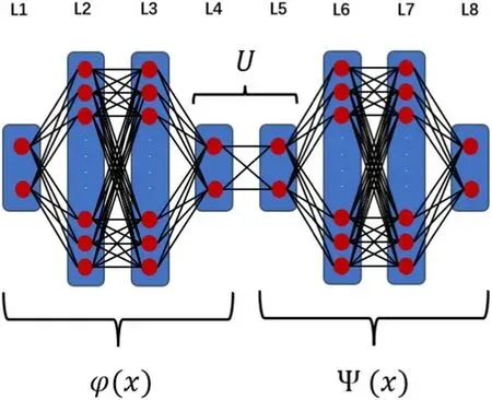
Figure 2.The modified network used in this paper.An evolutionary structure is added to advance the output of the encoder by one time step forward,just as the Koopman operator U does in this reduced representation.
Compared to the traditional auto-encoder,the architecture of the neural networks used in this paper is adapted to the current purpose and displayed in figure 2,where φ(x)denotes the encoder and ψ(x) the decoder as before.An evolutionary structure U is added and acts on the encoded data,representing the action of the Koopman operator on a minimal invariant subspace.
In fact,if the eigenvalue λ is real,one node could be used in each layer of U instead of two nodes as displayed in figure 2.In that case,obviously φ(x) encodes the corresponding eigenfunction and the weight between the two layers of U is just λ,the eigenvalue.Multiplication with λ is just the action of the Koopman operator on the eigenfunction.For complex eigenvalues,two nodes are needed in each layer of U as shown in figure 2.The four weights between these two layers could be written as a matrixwhere the values of a and b are real,which determine the eigenvalue pair a±ib,generally depicting a spiralling motion in the phase space.A pure rotation results only if a2+b2=1 which is guaranteed by the repeated application of U to φ(x)in practice as will be seen in the following numerical examples.It is worth noting that in the evolutionary structure U,layer L5 does not employ an activation function to ensure a proper simulation of the linear action of the Koopman operator on its eigenfunctions.
The above evolutionary structure deals with one mode or one pair of conjugate modes.As we will see later on,if more modes are involved,similar structures need to be juxtaposed to represent this increased complexity.The number of modes needed is learned by repeated trials and the necessity of adding extra modes is indicated by the magnitude of the loss function.
Previous works [37,38,41]mainly concentrate on the extraction of the approximately invariant subspace of the Koopman operator so there is not much constraint on the weight or size of the evolutionary structure K of the autoencoder.So,a lot of weights could enter the construction,which may bring extra uncertainty and instability in the training especially if the dimension of the invariant space goes high [52].In the current manuscript,the eigenfunctions are extracted directly by the auto-encoder step by step.The most important one is the first to obtain and then the second and so on,in contrast to most other computations [43,44].With the current approach,the size of the neural network,as well as the number of parameters,could be effectively reduced to avoid possible overfitting or trapping in local minima[41].Because the auto-encoder implements nonlinear reconstruction [45]rather than linear combinations of given basis functions [40],a natural sorting of the eigenfunctions could be defined according to the order of their birth,exercising the concept—what you see is what you get [42].
4.Results
In this section,we will apply the above formalism to several typical examples in classical mechanics with varying complexity.The first one is an over-damped oscillator which is described by a 1-d linear equation and the dynamics are a simple exponential decay.Then we go on to the well-known Van der Pol system which executes a periodic motion with driving and dissipation.These two examples are characterized by one eigenvalue (pair) of the Koopman operator as will be seen in the following.The other two examples involve two or three coupled oscillators described with the Kuramoto model.With two oscillators,very often,the motion is quasi-periodic which has two basic frequencies while The three-oscillator system could become chaotic with a broad band of frequencies emerging.In both cases,nevertheless,a few eigenvalues and eigenfunctions could be found which are sufficient to reconstruct the original dynamics fairly well with the help of the decoder.
4.1.One over-damped linear oscillator
As a test,we first study an over-damped oscillator with the inertia term ignored,described with a simple linear equation

which has an exponentially decaying solutionx(t)=x0exp(-(t-t0)),where x0=x(t0).The decay rate η=1 also appears in the exponent of the eigenvalue of the Koopman operatorλ=exp(nηΔt),where n is an integer and Δt is the evolution time step.It is easy to check that in this case,the corresponding eigenfunction is simply φ(x)=cxnwith c being an arbitrary constant.
The given time series starts from x=19.03 with Δt=0.1 and we take the first 100 points for training.The encoder consists of two hidden layers with 40 and 20 neurons and the decoder is a mirror image with two layers containing 20 and 40 neurons.The following loss function is used


Figure 3.A comparison of the Koopman analysis in equation(6).(a)The leading eigenfunctions obtained by the traditional DMD method(‘Koopman’)and by the auto-encoder(‘R’).(b)The original and the reconstructed trajectory of the autoencoder.
where x1is one part of the time series and x2is the time series after one time step Δt.The subscript‘MSE’denotes the mean square error.In the current case,the eigenvalue of the system is real,so there is only one neuron in each layer of the evolutionary structure.The calculated exponent is=1.005,very close to the exact one η=1.Figure 3 compares the eigenfunctions obtained by the auto-encoder and by the traditional DMD method(equation(5),with natural basis)which obtains a decay exponent of=0.998.The original and the reconstructed trajectory are also compared and match well in figure 3(b).It is seen that the eigenfunction obtained by the encoder is in good agreement with that obtained by the traditional DMD method,which seems to be close to y=-x,an exact eigenfunction.The value of the loss function is 1×10⁻⁶,which hints the accuracy of the approximation.
4.2.The Van der pol system
In the previous example,the system is linear and characterized by a simple exponential decay.Here,we consider the Van der Pol equation

which is proposed by Dutch physicist Van der Pol in 1928 to describe the electron tube oscillator of an LC circuit[53].This equation has both driving and dissipation terms competing with each other and as a result,a general solution approaches a unique stable limit cycle.It has become a prototype of stable nonlinear oscillation in mathematical physics.When α=0,it describes a simple linear oscillator.At small positive α,a limit cycle with radius~2 appears which continues to exist but deforms with α increasing.
On the limit cycle,the eigenvalues of the Koopman oscillator are characterized by complex pairsλ=exp(nωΔt),where ω=2π/T with T being period of the limit cycle.In order to deal with the system with different α values,we design a loss function


Figure 4.The leading eigenfunction obtained with the traditional DMD method (denoted by ‘Koopman’ corresponding to the eigenvalue 0.9959±0.0998i)and with the auto-encoder(denoted by‘R’ corresponding to 0.9951±0.0997i) for the Van der Pol equation (8) at α=0.1.The function is defined on a limit cycle given by the sampled discrete points,and the real and the imaginary part of the eigenfunction are marked here for each point.
with an adjustable parameter n,representing the forward time steps for comparison of the Koopman and the true trajectories,which is supplied to ensure the reconstruction accuracy.Here,y1is part of the observed time series and yi+1is the sequence after time iΔt.As the eigenvalue is complex,we put two neurons in each layer of the evolutionary structure as discussed in the previous section.
At the weak nonlinearity α=0.1,the limit cycle is close to a circle in the phase space and the time series starts from(1.76,0.99) with Δt=0.1.The period of the limit cycle is found to be T=6.29 which gives a frequency ω=0.9989.The first 1000 points of the time series are used for training an auto-encoder similar to what is shown in figure 2.Since the parameter is small,n=1 in equation (9) is good enough for the extraction of the most important eigenvalues.The obtained eigenvalue is=0.9951 ±0.0997i,which is very close to=0.9959 ±0.0998i,the eigenvalue calculated by the traditional DMD method.They both match well with the t heoretical valueλ=exp (iωΔt)~0.9950 ±0.0997i.The value of the loss function,5×10-5,indicates the accuracy.
Figure 4 compares the leading eigenfunction obtained with different methods.From the figure,it is easy to see that the eigenfunction obtained with the auto-encoder is highly consistent with that of the traditional DMD method,which signals the effectiveness of our method.Also,we found that the method is not sensitive to the initial values of a and b.
At α=1.5,the periodic orbit is quite distorted so that high-order harmonics become significant.The minimization with n=1 leads to a very irregular structure in the phase space since with α increasing,the system becomes very nonlinear and the auto-encoder easily falls into some local minimum.Thus,we need sufficient constraints on the autoencoder to procure the correct result.But n cannot be too large,either.Very large n makes the computation tedious and ineffective.The limit cycle is found to have the period T=7.08 so that ω=2π/T=0.8875.For the orbit data with the initial point (-0.806,1.212) and Δt=0.0708,when n=20 is used,the auto-encoder extracts the important eigenvalue=0.9981 ±0.0627i,which compares good with the one=0.9980 ±0.0626i from the DMD method(figures 5(c),(d)).They are both very close to the theoretical valueλ=exp (iωΔt)~0.9980 ±0.0628i.The value of the loss function is now 4×10⁻⁴,which indicates that the actual and the reconstructed trajectory almost overlap as depicted in figures 5(a),(b).
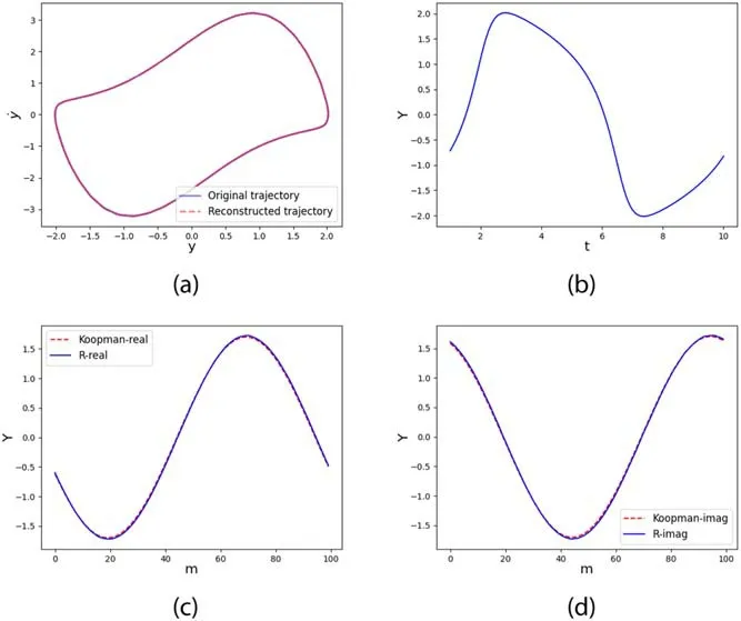
Figure 5.The trajectory reconstruction and the eigenfunction with λ~0.9980±0.0628i at α=1.5.(a) The original and the reconstructed cycle in the phase space.(b)The evolution of the real part over time.The real (c) and the imaginary (d) part of the eigenfunction,obtained with the traditional DMD and with the autoencoder.The horizontal axis is the index of sampling points.In this and subsequent figures,‘Koopman-real’ and ‘Koopman-imag’correspond to the real and imaginary part of the eigenfunction with the traditional DMD method,and ‘R-real’ and ‘R-imag’ to those with the auto-encoder.
4.3.Two coupled phase oscillators
In the above example,the asymptotic motion is relatively simple,residing on a one-dimensional curve.Below,we study coupled oscillators with more intricate dynamics such that two or more basic frequencies are needed to reconstruct the dynamics.
A typical example of high-dimensional nonlinear systems is the system consisting of coupled oscillators that exists ubiquitously,ranging from human circadian clocks [54]and sleep-wake cycle [55]in biology to laser arrays [56],microwave oscillators [57],superconducting Josephson junctions[58]in physics and engineering.Inspired by Winfree’s research[59],Kuramoto proposed his famous phase oscillator model in 1975 [60],in which each oscillator has a generic frequency but is also coupled to others with sinusoidal terms involving phase differences.Kuramoto model was initially used to describe biological or chemical oscillators,and later find applications in very wide contexts [61–63]since it is a general model to describe the synchronization behavior of coupled systems.In the following,Kuramoto model is used to demonstrate the validity of the above Koopman analysis.
First,we check two coupled phase oscillators with the equation of motion being

where ω1,ω2are generic frequencies of the two oscillators and K1,K2are two coupling constants.We will take the two incommensurate frequencies ω1=1,ω2=for example in the calculation below.
For K1=K2=0,the motion is quasi-periodic and densely fills a bounded region in phase space.The time series start atwith Δt=0.1,the first 1000 points of which are used as the training data.Because of the periodicity of angles,for convenience,we change the input from(θ1,θ2)to the new variablez=(s in (θ1),cos (θ1),sin(θ2),cos (θ2)).In the training,the following loss function is used

where n marks the number of steps in the observation data and p marks that in the eigenfunction for comparison.The functions φk's are different from Koopman eigenfunctions and Ukas the reduced Koopman operator acting specifically on the kth eigenfunction.All these eigenfunctions are encoded by different encoders but decoded by the same decoder.The symbol z1denotes one part of the time series and zm+1is the sequence after m time steps.
At K1=K2=0,the motion is quasi-periodic with two incommensurate frequencies.We take n=60,j=2 and p=4,α1=α2=1000 in the loss function equation (12).Two pairs of eigenvalues=0.9950 ±0.0998i and=0.9904 ±0.1388iare obtained and are in good comparison with those by the traditional DMD method,=0.9949 ±0.0989i and=0.9924 ±0.1404i.Both agree well with the exact valueλ1=exp (iω1Δt)=0.9950 ± 0.0998i andλ2=exp (iω2Δt)=0.9900 ±0.1410i.The corresponding eigenfunctions,as well as the reconstructed trajectory,are plotted in figure 6,which shows nice agreement,being consistent with the small value of the loss function,1.9×10-4.In this case,the motion in the two dimensions is independent of each other.Two basic frequencies are sufficient to give an accurate description.

Figure 6.The Koopman eigenfunctions and the evolution trajectory of the two coupled oscillators at K1=K2=0.The real and imaginary parts of the four eigenfunctions obtained with the traditional DMD method (a) and with the autoencoder (b) with the eigenvalue 0.9950±0.0998i.(c),(d) are similar to (a),(b) but for the eigenvalue 0.9900±0.1410i.The original (e) and the reconstructed (f) trajectory with the x=sin (θ1),y=sin(θ2).
At K1=K2=0.1,the orbit becomes deformed and more frequencies chip in which may not be written as simple integer linear combinations of the two basic generic frequencies,since the two oscillators interact with each other and the trajectories become entangled,although the motion is still quasi-periodic.We need to change the weight of α1to emphasize the accuracy of system reconstruction and evolution,for example α2=1000,α1=10 000 are good enough.In fact,as long as the ratio of α1to α2is not too small,the computation remains reasonable.The unitarity of the Koopman operator is ensured by setting p=6 in the loss function equation (12).
By increasing the number of sought eigenfunctions,it is found that four of them can achieve good reconstruction.If the number is three,the reconstruction is possible but with poor accuracy.When it is over four,the result does not improve significantly.Therefore,we set j=4,which results in four pairs of fundamental eigenvalues=0.9877 ±0.1497i,=0.9973 ±0.1357i,=0.9926 ±0.1274i,=0.9891 ± 0.1107i,well matching those obtained by the traditional DMD method=0.9869 ±0.1461i,=0.9912±0.1351i,=0.9917 ±0.1285i,=0.9940±0.1112i.The corresponding eigenfunctions as well as the trajectory are displayed in figure 7.The value of loss function remains small,2.9×10-4.

Figure 7.The eigenfunctions and the trajectory of the two coupled oscillators at K1=K2=0.1.The real and imaginary parts of the four eigenfunctions obtained by the traditional DMD method and by the auto-encoder for the eigenvalues equal to 0.9877±0.1497i (a),(b),0.9973±0.1357i(c),(d),0.9926±0.1274i(e),(f),0.9981±0.1107i(g),(h).(i) and(j)plot the original trajectory and the reconstruction,where the x-and y-coordinate axis corresponds to sin (1θ)and sin (θ2),respectively.
Here,we are not sure if four frequencies are the true minimal set since both the orbit segment and the width of the neural network are always finite,resulting in unavoidable errors in computation.Nevertheless,the trajectory is well reproduced with the above four frequencies,which seems to indicate the simplicity of the underlying motion in some sense.This type of knowledge may not be easy to obtain with other approaches.
4.4.Three coupled phase oscillators
In previous examples,the motion is periodic or quasi-periodic.Here,we study a three-dimensional dynamical system consisting of three coupled oscillators,which has the equation of motion

where ωi's are intrinsic frequencies of the oscillators and Kij's are coupling constants.Depending on the values of the couplings and the initial conditions,the motion could be periodic,quasi-periodic or chaotic.In the following,we take the parameter values ω1=1,ω2=,ω3=,K11=K12=K21=K22=K31=K32=0.2.If starting with the initial point (1279.64,1455.93,1494.26),the motion is weakly chaotic with three Lyapunov exponents being (0.02,0,-0.17).One thousand points are used as the training data along a chaotic trajectory with Δt=0.05.We continue to use the loss function equation (12) with parameter values α1=10 000,α2=1000,n=60,p=6 and j=4.Still,the input is taken to bez=(s in (θ1),cos (θ1),sin (θ2),cos (θ2),sin(θ3),cos(θ3))to match the periodicity in the angle variable.
Similar to the previous case,the number of Koopman eigenfunctions included substantially influences the reconstruction of the dynamical system.When j=3 in equation (12) the reconstruction seems bad,while for j=4 the evolution trajectory could be reproduced quite precisely with an error of 4.1×10⁻⁵.For j=5,due to the increase in the number of parameters,the training sometimes falls into local minima and leads to failure.Even if this does not happen,the additional eigenvalue obtained by the new encoder is most often identical to the previous four.So,the reconstruction does not get better and we believe that j=4 is the most appropriate.It seems that in this way a fundamental set of eigenfunctions could be defined which is able to map out a long segment of the chaotic trajectory in a nonlinear manner.
The computed four pairs of Koopman eigenvalues=1.0029 ±0.0753i,=0.9977 ±0.0701i,=0.9971 ±0.0684i,=0.9986 ±0.0667iare very close to what has been obtained with the traditional DMD method:=0.9981 ±0.0748i,=0.9976 ±0.0698i,=0.9977 ± 0.0683i and=0.9987 ±0.0671i.The original trajectory is plotted in the phase space together with its reconstruction in figure 8 and they almost overlap each other.The real and imaginary parts of the corresponding eigenfunctions are also compared,which seem to be in good agreement although the orbit is weakly chaotic.

Figure 8.The original and the reconstructed trajectory of the three coupled oscillators.The blue line marks the original trajectory and the orange line is the reconstruction.The x-,y-,z-axis correspond to variables sin (1θ),sin (θ2) and sin (θ3).
It is well known that the chaotic motion has a broad band of frequencies that could not be reduced to linear integer combinations of a few basic frequencies in a rigorous way.However,in the current case,as the orbit is weakly chaotic,there remain several dominant frequencies that should be captured by our construction.Through the nonlinear mapping materialized by the decoder,other frequencies could be well approximated by linear combinations of these frequencies.The difference may not be large enough to generate a perceivable discrepancy in a finite segment of the orbit.
5.Discussion and conclusion
The Koopman operator transforms a nonlinear system in phase space into a linear one in functional space which serves as a powerful technique for computation and analysis of complex systems.However,in practice,it is difficult to select proper basis functions to realize this transformation that meets specific needs due to the possible high-dimensionality of observable space and the variability of the dynamics.Nevertheless,the resurgence of deep learning in 2006 [33]together with its wide application in natural or social science and engineering brings us new tools.The powerful representation capability of artificial neural networks (ANNs) is able to make any desired coordinate transformation as long as there are enough neurons.Interesting work has been started along this line with much success.But the robustness and the interpretability of the ANN and the determination of the most relevant eigenfunctions of the Koopman operator remains elusive.In addition,in this type of training,a large amount of representative training data and computational power are usually required [49,52],which may be difficult to obtain in certain fields such as in medical treatment.
In the current manuscript,we aim to find a set of important Koopman eigenvalues and their corresponding eigenfunctions based on one type of neural network—the modified auto-encoder.Since there is no need to choose basis functions,the efficiency and the numerical stability is greatly improved compared to the traditional DMD[29].At the same time,because of the minimization of the fitting error in the auto-encoder,it is no longer necessary to manually distinguish whether a Koopman eigenfunction is important or not as in the traditional method.In this way,the result of the encoder is highly interpretable and also the training becomes easier [37].
Admittedly,the auto-encoder is not perfect with obvious shortcomings as in general neural networks,such as the reliance on expert experience in the selection of hyper-parameters and the consumption of much computation power for the training.In addition,the results obtained by the autoencoder are accurate only in the close neighbourhood of orbital data and soon become useless away from the trajectory.Much work needs to be done to investigate the generalizability of the representation to other parts of the phase space or even to other parameters.
With the powerful representation capability and adaptable structure of the ANN,it is promising to extend application of the current technique to high-dimensional nonlinear systems,providing tools for the analysis of complex dynamical systems in different fields such as weather forecasting and epidemiology [64,65].With real data and new requirements,more efficient networks and better loss functions may be designed to accelerate the learning of key Koopman eigenfunctions [37,38].
Acknowledgments
This work was supported by the National Natural Science Foundation of China under Grant No.11775035,and by the Fundamental Research Funds for the Central Universities with contract number 2019XD-A10,and also by the Key Program of National Natural Science Foundation of China(No.92 067 202).
Appendix A.Method
We created our datasets by solving systems of differential equations in MATLAB using the ode45 solver.The neural network model is constructed on the TensorFlow framework[66]and trained with the Adam optimizer [67],and the learning rate is 0.001.We initialize each weight matrix W by the GlorotNormal method [52].Each bias vector b is initialized to 0.The activation function of each hidden layer used in all examples is ReLU,which may effectively avoid gradient saturation and accelerate the calculation.This activation function is also the most widely used one at present.Each model is trained for 100 000 epochs on a Nvidia RTX3090 GPU.
Appendix B.Selection of hyper-parameters
Hyper-parameters include neural network parameters,optimization parameters and regularization parameters.Neural network parameters include the number of layers,the number of neurons contained in each layer and the weights between different layers,etc.Optimization parameters include optimizer,learning rate,etc.Regularization parameters include regularization coefficients,etc.So far,there is no rule of thumb for the selection of hyper-parameters,which is more or less a combination of actual demand and prior experience[33].A general guideline is that more complex tasks require more hidden layers and more hidden layer neurons.
Similarly,the hyper-parameters involved in this paper,such as the number of hidden layers,the number of neurons in each hidden layer,α1,α2,n,t,j in the loss function,learning rate and other hyper-parameters are given out of experience.We cannot guarantee that the combination of these hyperparameters here is optimal,but it should be effective.One trick is that in order to improve the memory utilization of the computer,the number of neurons is usually set to 2nwhen the size of neural network is large [49,51].
杂志排行
Communications in Theoretical Physics的其它文章
- Preface
- Phase behaviors of ionic liquids attributed to the dual ionic and organic nature
- Chaotic shadows of black holes: a short review
- QCD at finite temperature and density within the fRG approach: an overview
- The Gamow shell model with realistic interactions: a theoretical framework for ab initio nuclear structure at drip-lines
- Effects of the tensor force on low-energy heavy-ion fusion reactions: a mini review