Hybrid Fault Diagnosis and Isolation for Component and Sensor of APU in a Distributed Control System

，，*，，，

1.Jiangsu Province Key Laboratory of Aerospace Power Systems，Nanjing University of Aeronautics and Astronautics，Nanjing 210016，P.R.China；

2.Aviation Motor Control System Institute，Aviation Industry Corporation of China，Wuxi 214063，P.R.China

Abstract: This paper addresses the gas path component and sensor fault diagnosis and isolation（FDI）for the auxiliary power unit（APU）.A nonlinear dynamic model and a distributed state estimator are combined for the distributed control system.The distributed extended Kalman filter（DEKF）is served as a state estimator，which is utilized to estimate the gas path components’flow capacity.The DEKF includes one main filter and five sub-filter groups related to five sensors of APU and each sub-filter yields local state flow capacity.The main filter collects and fuses the local state information，and then the state estimations are feedback to the sub-filters.The packet loss model is introduced in the DEKF algorithm in the APU distributed control architecture.FDI strategy with a performance index named weight sum of squared residuals（WSSR）is designed and used to identify the APU sensor fault by removing one sub-filter each time.The very sensor fault occurs as its performance index WSSR is different from the remaining sub-filter combinations.And the estimated value of the soft redundancy replaces the fault sensor measurement to isolate the fault measurement.It is worth noting that the proposed approach serves for not only the sensor failure but also the hybrid fault issue of APU gas path components and sensors.The simulation and comparison are systematically carried out by using the APU test data，and the superiority of the proposed methodology is verified.

Key words：auxiliary power unit（APU）；gas path fault；sensor fault diagnosis and isolation；packet loss model；Kalman filter

0 Introduction

It is well known that the auxiliary power unit（APU），an important subsystem of the aircraft，is a miniature gas turbine engine that is self-contained and requires no external energy［1］.APU provides power，gas，and hydraulic energy for the aircraft during the flight and restarts the engine in the event of an in-flight shutdown［2］.The operating condition should be supervised in real-time，and it guarantees the APU reliability and stability［3］.Sensor measure⁃ments are the primary sources of APU status infor⁃mation，and the accuracy of measurements is critical for APU control，performance monitoring，and di⁃agnostics.Due to the harsh working environments and variable operating conditions of the aircraft，the sensors are fault-prone parts［4］.Various failures of the APU control system result from inaccurate read⁃ings.Hard redundancy and soft redundancy are two primary ways to improve the sensor reliability of the APU control system.The additional devices are usually installed by hard redundancy，leading to a weight increase.Hence，this paper mainly focuses on soft redundancy.The estimated measurements from the mathematical model are drawn and re⁃placed with the fault sensor measurements in APU as the hard redundancy fails［5］.

The Kalman filter（KF）is a widely used meth⁃od to realize engine soft redundancy and it reduces the computational burden under the distributed con⁃trol system.Significant advances in distributed fil⁃ters research have been made since the early 1970s.The structure of distributed filters with multiproces⁃sors has been proposed.Each computing unit related to the node sensor was used to process the informa⁃tion obtained at all nodes，and each node got the overall results［6］.Furthermore，the architecture of a global filter with multiple sub-filters was developed and sub-filters were independent of each other.That the global filter completes the fusion of local results reduces the communication burden between sub-fil⁃ters［7］.To realize the diminution of the network communication burden，Ribeiro derived a recursive algorithm named sign of innovations-Kalman filter（SOI-KF）for distributed state estimation based on residual markers［8］.Safari et al.developed a novel sensor fusion method for multi-rate sensor network systems via a neural network approach to estimate state vectors［9］.Chen et al.proposed a finite time do⁃main federated Kalman filter algorithm to reduce the computation burden of filter and improve the sensor fault tolerance of multi-sensor network systems［10］.In the situation of a bias fault，Qiu et al.designed an intelligent covariance online sequence extreme learn⁃ing machine（COSELM）algorithm to tackle the signal reconfiguration problem of the sensor［2］.

GAO proposed a distributed extended Kalman filter（DEKF）algorithm with one main filter and five sub-filters to estimate health parameters［11］.Each sub-filter was designed independently and com⁃puted in parallel［12-13］.The pre-obtained local results were transmitted to the main filter for information fusion to get a global posterior estimation.The main filter assigned information to the sub-filters and state estimation fed back to sub-filters based on the global estimation［14］.A packet loss model was introduced to reflect the random occurrence of packet loss in measurements transmission from local sensors to the main filter［11，15］.The likelihood of packet loss for each sensor was considered to be the same and con⁃stant at all times［11］.A state receiving matrix was constructed according to the measurement transmis⁃sion conditions after the packet loss probability was set.An improved DEKF algorithm with a packet loss model was presented by taking the state receiv⁃ing matrix into account.

The estimated value of the sensor was calculat⁃ed by the DEKF algorithm，and a performance in⁃dex named weight sum of squared residuals（WSSR）was used to identify the APU sensor fault［16-18］.The sensor was faulty as its WSSR was different from the remaining sub-filter combina⁃tions，and the estimated value of the sensor at a fault-free time was used to replace the fault value.Then，compared with the original WSSR val⁃ues［19-21］，all the WSSR values after isolation were less than the threshold，and the isolation was regard⁃ed as successful.

In this paper，due to the extreme sensor work⁃ing environments such as high temperature，five sensors are measurable and employed to estimate two flow capacity coefficients that are not obtained directly.The measurements are rotation speed sen⁃sor，compressor outlet temperature sensor，com⁃pressor outlet pressure sensor，turbine outlet tem⁃perature sensor，and turbine outlet pressure sensor.While the two flow capacity coefficients are com⁃pressor flow coefficient and turbine flow coefficient.Different from the research mentioned above，the in⁃novation of this paper lies in a new application of the DEKF algorithm with random packet loss on the APU.The DEKF algorithm estimates the air path flow capacity coefficients not only in normal condi⁃tions，but also in the situation of sensor failures.Sin⁃gle and dual sensor faults are considered in the esti⁃mation process as two typical failure modes.The simulation results show that the isolation module eliminates sensor faults in a timely and effective manner in both types of sensor failures and ensure that the estimation of flow capacity coefficients re⁃mains correct and unaffected from the faulty sensors.

The roadmap of this paper is as follows.In Sec⁃tion 1，the nonlinear dynamic model of APU is in⁃troduced.Two flow capacity coefficients are em⁃ployed to characterize the gas path flow characteris⁃tics of APU components and the structure of adap⁃tive model with Kalman filter bank is introduced briefly.Section 2 presents the DEKF algorithm with a packet loss model.Sensor fault isolation logic in the situation of single sensor fault or dual sensor fault is introduced in Section 3.Structure of APU sensor fault detection and isolation system and work⁃flow of fault isolation mechanism are presented.In Section 4，gas path fault，sensor fault and hybrid fault are simulated and discussed respectively to ver⁃ify the feasibility of diagnosis and isolation.Finally，some conclusions are summarized in Section 5.

1 APU Model and Problem Setup

This paper focuses on a single-spool APU.Gas path components of the APU include inlet，com⁃pressor，combustor，turbine，and nozzle.The APU nonlinear dynamic model is written by TMATS and works in SIMULINK.And it is established on the basis of component level engine modeling theories.Firstly，the mathematical model of each component is built according to the characteristics of APU com⁃ponents and design point parameters.Then，the co⁃operative working equations of components are es⁃tablished based on the principles of power balance and rotor dynamics.Finally，the numerical value it⁃eration algorithm is employed to solve the equations to obtain the parameters of each working section.The flight condition parameters of the established model are flight altitudeH，Mach numberMa，and inlet temperature.The nonlinear dynamic model of the APU is presented as

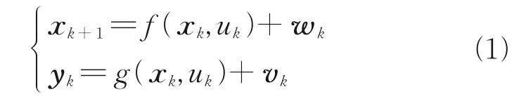
wherekis the time index，andxk，ukandykdenote the state variables，input variables and sensor mea⁃surements at timek，respectively.The model input variable is combustion chamber fuel flowWf.The state variables of the model include rotation speednand flow capacity coefficientsh，x=[n，hT]T.wkandvkrepresent uncorrelated system noise and mea⁃surement noise respectively，meetingwk～N(0，Q2)，vk～N(0，R2).HereQandRare the noise covariance matrices of system noise and measurement noise，respectively.f（·）andg（·）are the state transition function and measurement function of the APU model，respectively.The output parameters include rotation speedn，compressor outlet temperatureT3，compressor outlet pressureP3，turbine outlet temperatureT5and turbine outlet pressureP5.

Due to the limitation of the number of sensors and the internal structure of the established APU model，only the flow capacity coefficients are cho⁃sen to be estimated accurately.Two flow capacity coefficients characterize the gas path flow character⁃istics of APU components completely.Considering that the performance of gas path components will in⁃evitably change during the actual operation of the APU，the flow capacity coefficients are introduced to characterize the flow capacity degradation caused by individual performance differences or operation time of the APU.The flow capacity coefficients of gas path componentshare presented ash=[CW，TW]T，which are defined as

whereAis the actual flow of components andA*the ideal value.The subscript 1 represents the compres⁃sor and subscript 2 the turbine.The parametersCWandTWare the flow capacity coefficients of com⁃pressor and turbine，respectively.By expanding the state variablesx=[n，hT]T，the corresponding APU model in Eq.（1）is the expanded model.

APU may have gas path faults or sensor faults，or both.It is very important to judge whether the changes in sensor measurements are caused by gas path faults or sensor faults.Firstly，in the situation of gas path faults，this paper will verify the estima⁃tion accuracy of flow capacity coefficients without adding sensor faults.Then，gas path faults and sen⁃sor faults are added at the same time.All sensor faults are eliminated as long as the threshold is set appropriately，and the injected gas path fault is still estimated correctly.The centralized Kalman filter（CKF）processes all the sensor measurements in one Kalman filter，so the sensor fault tolerance is poor.When a sensor fails and outputs error measure⁃ments，the CKF needs to be terminated and rede⁃signed to select the correct sensors，so the continu⁃ous operation of the filtering algorithm is difficult.In comparison，the sensor fault tolerance of DEKF is higher.When a sensor fails，the DEKF only needs to take measures to isolate the faulty sub-filter，and the filtering algorithm is carried out continuously.Fig.1 shows the structure of an adaptive model with Kalman filter bank，whereyare the sensor measure⁃ments，g(x，u) outputs of APU model，and Δythe difference ofyandg(x，u).

Fig.1 Adaptive model structure based on Kalman filter bank

Fig.1 presents an adaptive model with the Kal⁃man filter bank which contains six Kalman filters and each one uses the DEKF algorithm.In every Kalman filter，each sub-filter only corresponds to one sensor，and this simplifies the data transmission and is not easy to make mistakes.The transmission structure is miniaturized and the weight of hardware equipment is reduced.A single sensor also minimiz⁃es the impact of noise interference.Compared with the traditional CKF，distributed filters adopt a paral⁃lel processing structure and share the computational burden of the main filter.

2 DEKF Algorithm with Packet Loss Model

2.1 DEKF algorithm

For a multi-sensors system such as the APU model，sensors are grouped to divide into different subsystems.Each sensor corresponds to a sub-fil⁃ter，which is designed independently and calculated in parallel.The results obtained from sub-filters are transmitted to the main filter for information fusion and global posteriori estimation is obtained.The main filter will allocate information to sub-filters ac⁃cording to the global posteriori estimation and reset the sub-filters’state.Denote the total number of sub-filters asM，the calculation process of DEKF is written as follows.

（1）Posteriori estimation resultsx0|0andP0|0are initialized.

（2）Main filter information distribution is given by

（3）Sub-filters calculate the local filtering re⁃sults.

The calculation process of Jacobian matricesAandCis as follows

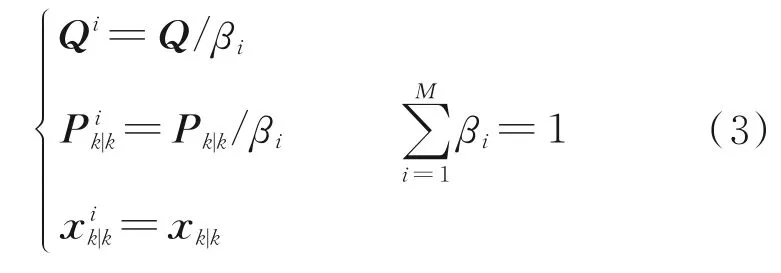
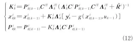
whereiis the sub-filter numberandRidenote the Kalman gain，the Jacobian matrix，out⁃put variables and noise variance matrix related to the sub-filteri，respectively.The sub-filter is designed according to the above DEKF algorithm.

（4）Main filter information fusion is given by

（5）Letk=k+1，and repeat from step（2）until the filtering process is completed.

2.2 Packet loss model

In the process of data transmission，the prob⁃lem of flow capacity coefficients estimation in the sit⁃uation of partial data loss is considered.For packet loss in data transmission，it is modeled by an inde⁃pendent identically distributed variablewhich satisfies the 0-1 distribution.The probability distri⁃bution is written as

wheregi(xk，uk) is the nonlinear subsystem corre⁃sponding to the sub-filteri，andare the subsystem state receiving matrix and the measured noise vector respectively.Eq.（5）is modified as

The structure of DEKF algorithm with packet loss model used in the APU model is shown in Fig.2.

Fig.2 Structure diagram of DEKF algorithm with packet loss model

3 Sensor Fault Diagnosis and Isola⁃tion Logic

To alleviate the influence of faulty sensors，a sensor fault diagnosis and isolation system based on the Kalman filter bank is established，and the design principle is discussed.The APU sensor fault diagno⁃sis and isolation system is mainly composed of an APU model，a measurements input module，a Kal⁃man filter bank module，a fault diagnosis and isola⁃tion mechanism module，and a fault sensor reconfig⁃uration module.The system is shown in Fig.3.

Fig.3 APU sensor fault diagnosis and isolation system

In Fig.3，yis the APU sensors measurements，uthe input control value，g(x，u) the outputs of APU model，g1(x1，u)the estimated values of mea⁃surements in Kalman filter 1，andg5(x5，u)the esti⁃mated values of measurements in Kalman filter 5.WSSR1 is the WSSR generated by Kalman filter 1，dWSSR1 is the dWSSR generated by Kalman filter 1，and others are the same.In the Kalman filter bank，the structure of Kalman filter 0 is the same as the one in Fig.2.Kalman filter 0 employs all 5 sen⁃sors to generate the WSSR which contains all the sensor fault information.Kalman filter 1 is the one without sub-filter 1，and its input sensor measure⁃ments named subset 1 of measurements include four sensors except for the rotation speed sensor.As a re⁃sult，the WSSR generated by Kalman filter 1 con⁃tains sensor fault information of four sensors except for the rotation speed sensor.The same is true for other Kalman filters.The workflow of the fault diag⁃nosis and isolation mechanism is shown in Fig.4.

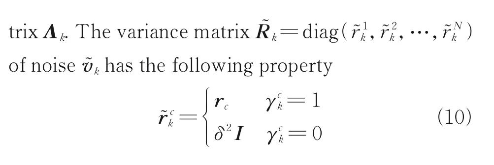
When an APU sensor fails，the sensor mea⁃surement and the Kalman estimated value must not be consistent and these filter residuals containing the information of sensor fault will also change.The fil⁃ter residuals are normalized by the filter weight sum of squared residualseiT(Σi)-1ei，which are named as the fault indication signal WSSR.HereΣi=[diag(σi)]2，σiis the standard deviation of theith sensor subset，andeithe difference between the sen⁃sor measurement and the estimated value.

Since the measurement noise of the sensor is Gaussian white noise with zero mean value，eihas the same property as the measurement noise.The fault isolation principle is that each Kalman filter is used to monitor a specific sensor and is designed based on fault-tolerant technology.When a sensor fails，the Kalman filter monitoring this faulty sensor only uses the measurements of other fault-free sen⁃sors，and the corresponding WSSR remains small.On the other hand，the others are Kalman filters in which the used subsets of measurements contain faulty information，and the related WSSR will in⁃crease and eventually exceed the preset threshold.Therefore，the faulty sensor is detected by setting a reasonable threshold and analyzing WSSR.

As shown in Fig.4，different subsets of the measurements are used as the input to the related Kalman filter.The estimated values of the corre⁃sponding sensors and WSSR are obtained by the Kalman filter bank.Through the analysis of WSSR，the fault isolation mechanism makes a judg⁃ment.The measurement is directly sent to the APU control system while the sensor is fault-free，so the APU continues to operate safely and reliably.In the situation of sensor fault，the fault reconfiguration module is informed of the diagnosis result obtained by the fault isolation mechanism，and it reconstructs the corresponding fault sensor measurement.

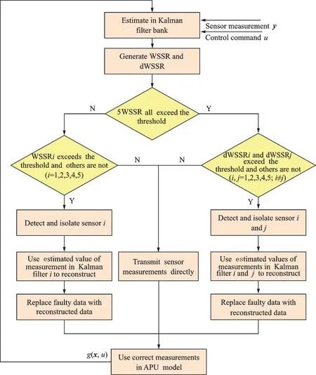
Fig.4 Workflow of APU fault diagnosis and isolation mechanism

A dual sensor fault refers to two sensors failing simultaneously.For the reason that more than one sensor has failed，the original fault diagnosis and iso⁃lation logic designed for a single sensor fault are no longer applicable.When a dual-sensor fault occurs，the five WSSR related to the five Kalman filters which sequentially remove one sensor will all ex⁃ceed the threshold.It is easy to find that a dual-sen⁃sor fault has occurred by the analysis of WSSR，but it is impossible to tell which sensors have failed.For this reason，the diagnosis and isolation logic em⁃ployed for dual-sensor fault is redesigned.Because the WSSR is the sum of residuals of the measured and estimated values of different sensors，it is cumu⁃lative naturally.The WSSR value of a dual-sensor fault should be higher than that of a single sensor fault，so an additional filter that does not remove any of the sensors is employed to record all the faulty sensor information by related WSSR.The WSSR output from this additional filter is named WSSR0.Eq.（13）is given by

where dWSSRiis the difference between WSSR0 and WSSRi.

That the corresponding dWSSRiwill signifi⁃cantly exceed the threshold is the same in the situa⁃tion that theith sensor fails or a dual-sensor fault oc⁃curs，and the location of the faulty sensors is deter⁃mined.When it is detected that all five WSSR are higher than the threshold，the saved APU sensor da⁃ta is simulated again after the current simulation to isolate the dual-sensor fault.The schematic diagram of dual-sensor fault diagnosis is shown in Fig.3.

4 Simulation and Discussion

4.1 Gas path fault diagnosis

In this paper，n，P3，T3，P5andT5are selected as the measurements to be monitored by the APU.The appropriate noise whose corresponding covari⁃ance isR=[0.001 52，0.001 52，0.001 52，0.001 52，0.001 52]［2］is added into the model.

The degradation is simulated in 60 s.The sam⁃pling time of the examined APU is set to 0.015 s and the total number of sampling steps is 4 000.A packet loss model with the packet loss probability of 10% is employed to reflect the data packet loss phe⁃nomenon.At the design point（Ma=0，H=0 km），the APU starts from the nominal condition，and flow capacity coefficients magnitudes at this condi⁃tion are 1.Two anomaly modes simulation of APU gas path are carried out as follows.

（1）Abrupt degradation mode of gas path：Flow capacity coefficients deviate from their normal value suddenly.In the APU model，the situation that two flow capacity coefficients shift from their nominal values is presented as follows：-2% onCW，+1% onTW［11］，and the occurring time of 1 s.

（2）Gradual degradation mode of gas path：Two flow capacity coefficients synchronously and linearly move to their terminal magnitudes from their nominal values in 60 s at the design point as fol⁃lows：-2% onCW，and +1% onTW［22］.

After testing，the flow capacity coefficients of the APU model are estimated in the range of about 0.98 to 1.02 due to the limitation of APU model structure.The results of flow capacity coefficients estimation at two typical modes are shown in Figs.5 and 6，where the red and black lines represent the true and estimated values，respectively.

From Figs.5 and 6，the gas path performance degradation is quickly tracked and accurately esti⁃mated at two typical modes in 60 s，and the DEKF combined with a packet loss model is tested to be ef⁃fective in the case of abrupt or gradual degradation.

Fig.5 Abrupt degradation simulation of gas path compo⁃nents

Fig.6 Gradual degradation simulation of gas path compo⁃nents

4.2 Sensor fault diagnosis

4.2.1 Single sensor fault diagnosis

The total simulation time is 60 s.It is assumed thatn（Sensor 1）fails from 2.02 s to 4.02 s，P3（Sensor 2）from 12.02 s to 14.02 s and from 17 s to 17.07 s，T3（Sensor 3）from 24.02 s to 26.02 s，P5（Sensor 4）from 36.02 s to 38.02 s，andT5（Sensor 5）from 48.02 s to 50.02 s.The sensor failure types are intermittent bias failures，and the fault ampli⁃tude is 2%.

The reasonable threshold is the key to the whole sensor fault isolation system.On one hand，too large thresholds would lead to missed diagnosis and many faults are not detected.On the other hand，setting a too small threshold is easy to mis⁃take the normal disturbance of some measurements as a fault.At the design point，the detection thresh⁃old is taken as 25 in the situation that sensors are no fault.The simulation results are shown in Fig.7.

It is worth noting that in Fig.7，except that the WSSR related to the fault sensor in the correspond⁃ing fault time still maintains a small value，the WSSR related to other sensors begin to increase in the above fault time and exceed the set detection threshold.Therefore，the fault isolation mechanism detects the occurrence of the bias fault and find which sensor has failed timely and accurately.

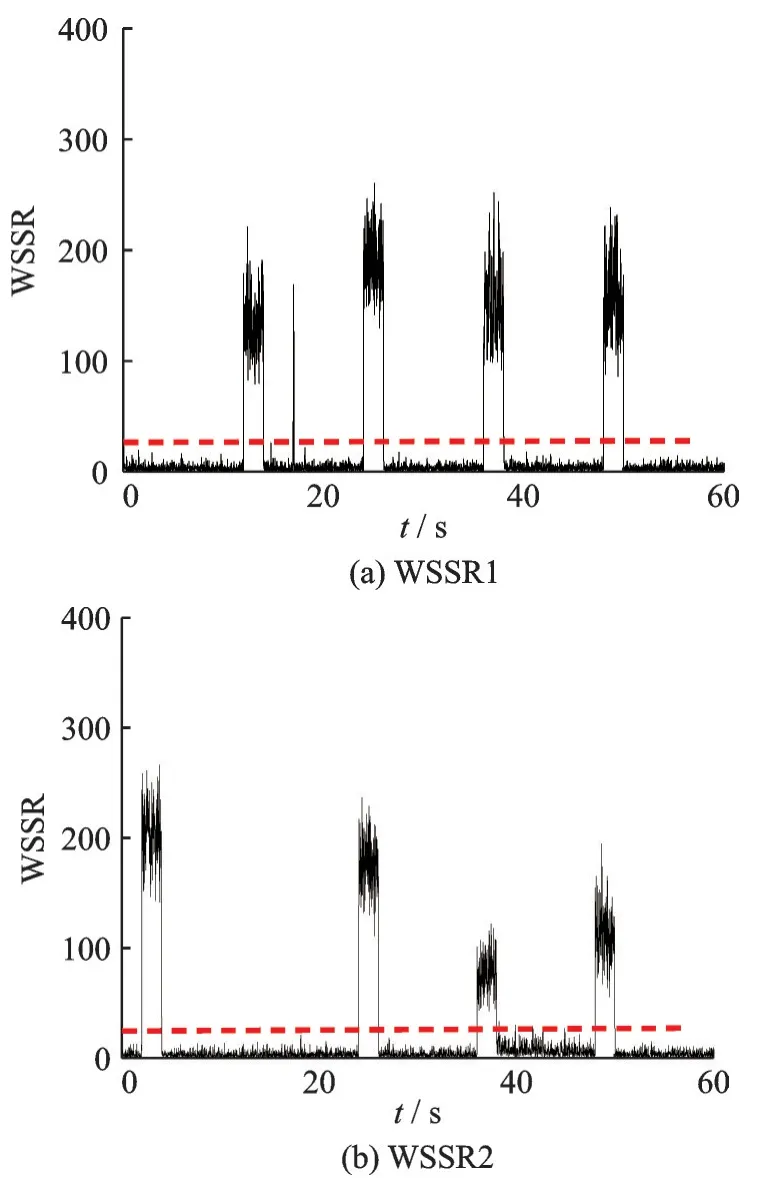
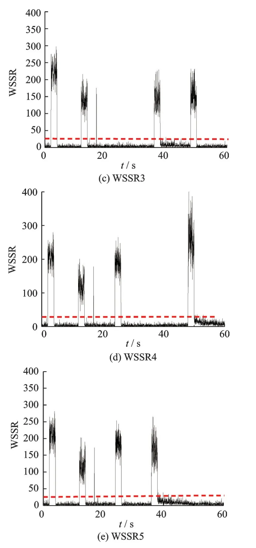
Fig.7 WSSR in the case of single sensor fault simulation

To avoid the usage of the wrong measure⁃ment，the sensor fault detection and isolation sys⁃tem combined with the Kalman filter bank replaces the faulty measurement with the estimated value of sensor measurement output from the Kalman filter which does not use the faulty sensor.Kalman filter 0 has all of five sensors and presents all the sensor fault information.WSSR0 related to Kalman filter 0 before and after isolation are shown in Fig.8.

From Fig.8，WSSR0 is all smaller than the threshold in 60 s after isolation and the reconstruct⁃ed value effectively avoids the Kalman filter bank from using the wrong measurement at the beginning of the fault.

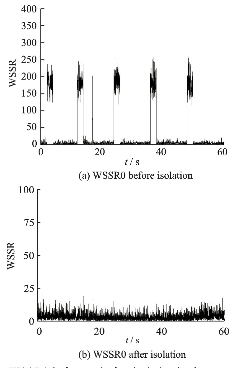
Fig.8 WSSR0 before and after isolation in the case of sin⁃gle sensor fault simulation

The fault amplitude has a great impact on the isolation accuracy.Generally speaking，the larger the amplitude is，the easier the fault is detected.The smaller the amplitude is，the easier the fault mixes with the measurement noise.In the situation that the amplitude is too small，likely the fault will not exceed the threshold at the beginning，so the fault isolation mechanism will still bring in the wrong value.Fig.9 shows the state of sensor fault isolation failure when each sensor tested is just at the lower limit of fault amplitude of isolation failure.

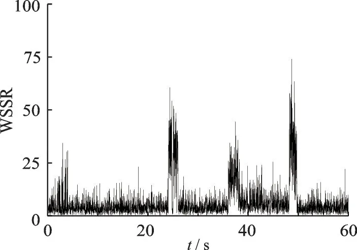
Fig.9 WSSR0 in the case of single sensor fault isolation failure

From Fig.9，except forP3sensor，the other sensors fail in isolation，but their lower limits of iso⁃lation failure are different.Table 1 shows the lower limit of isolation failure for each sensor and the isola⁃tion accuracy when the fault occurs.

Table 1 Amplitude lower limit and accuracy of each sen⁃sor isolation

4.2.2 Dual sensor fault diagnosis

In the case of dual-sensor fault，the total simu⁃lation time is set to 60 s.n（Sensor 1）fails from 12.02 s to 50.02 s，P3（Sensor 2）from 19.02 s to 50.02 s，so a dual-sensor failure occurs from 19.02 s to 50.02 s.All fault types are bias faults and have an amplitude of 2%.The simulation results of the WSSR are shown in Fig.10.

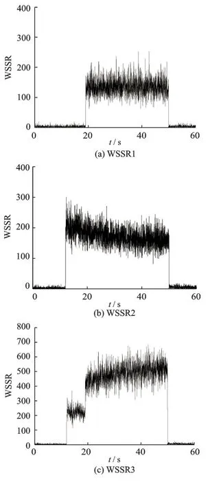
Fig.10 WSSR in the case of 2% bias faults of n and P3 sen⁃sor simulation

From Fig.10，the five WSSR from WSSR1 to WSSR5 all exceed the threshold value 25 from 19.02 s to 50.02 s when the dual sensor fault oc⁃curs，so it is impossible to tell which sensor is actu⁃ally faulty.The WSSR0 from 19.02 s to 50.02 s is obviously larger than that of a single sensor fault oc⁃curring from 12.02 s to 19.02 s，so it is possible to use the cumulative nature of the WSSR.The WSS⁃Riis subtracted from WSSR0 containing all fault in⁃formation to obtain the corresponding dWSSRi.dWSSR simulation results are shown in Fig.11.

Fig.11 dWSSR in the case of 2% bias faults of n and P3 sensor simulation

The threshold for dual-sensor fault is set to 100.Only the values of dWSSR1 and dWSSR2 ex⁃ceed the threshold at the corresponding time of fault occurrence，and the rest of the dWSSR are less than the threshold.BothnandP3sensors fault con⁃ditions are diagnosed from 19.02 s to 50.02 s after the onset of dual sensor fault.After isolation，the WSSR0 simulation result is shown in Fig.12.

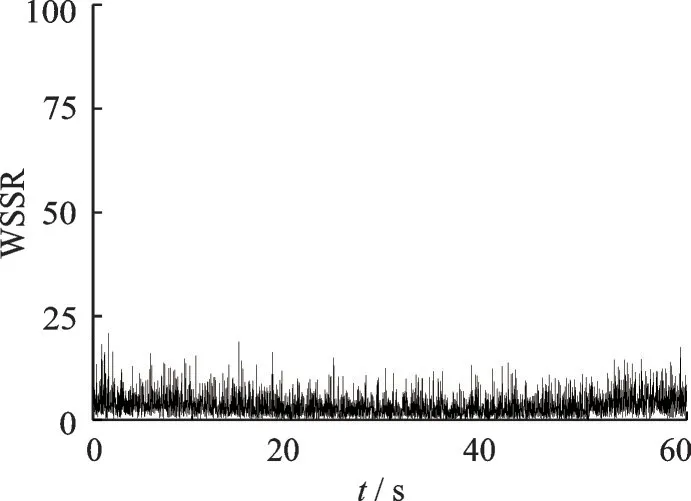
Fig.12 WSSR0 after isolation in the case of 2% bias faults of n and P3 sensor simulation

It is easy to find that the reconstructed WSSR0 is less than the threshold in 60 s and the dual-sensor fault is successfully diagnosed and isolated.

4.3 Hybrid fault diagnosis

Sensor fault diagnosis simulation has been car⁃ried out to verify the feasibility of the Kalman filter bank on it.Then，sensor faults and gas path degra⁃dation are added simultaneously into the APU to more intuitively reflect the effect of sensor isolation，and the flow capacity coefficients tracking results are drawn before and after isolation.

4.3.1 Single sensor and component fault

In addition to the above sensor faults added in the single sensor fault situation，gas path abrupt deg⁃radation mode and gas path gradual degradation mode are employed to the APU respectively.The flow capacity coefficients estimation results of two anomaly modes before and after isolation are shown in Fig.13 and Fig.14，respectively.

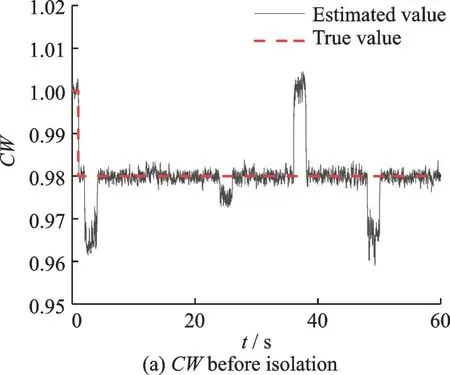
Fig.13 Flow capacity coefficient estimation in the case of single sensor fault with abrupt degradation of gas path

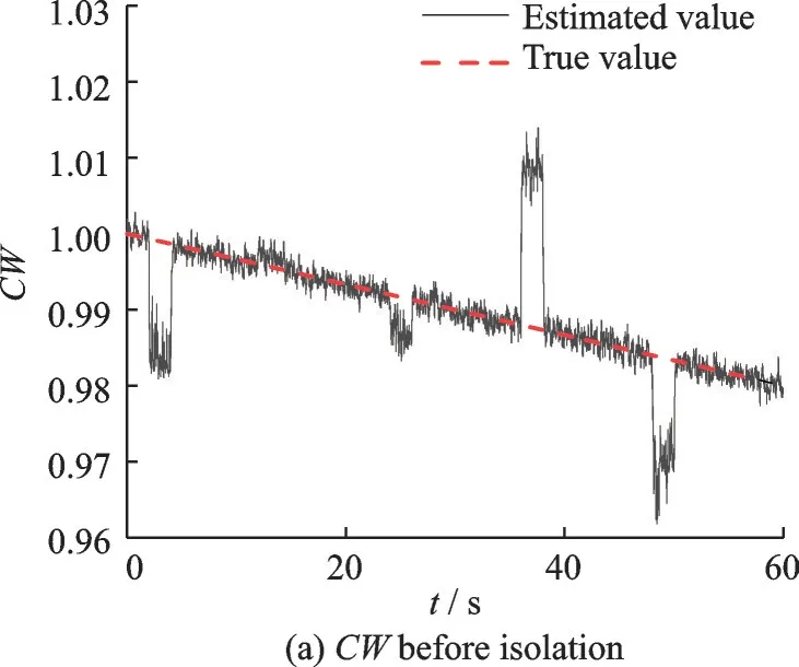
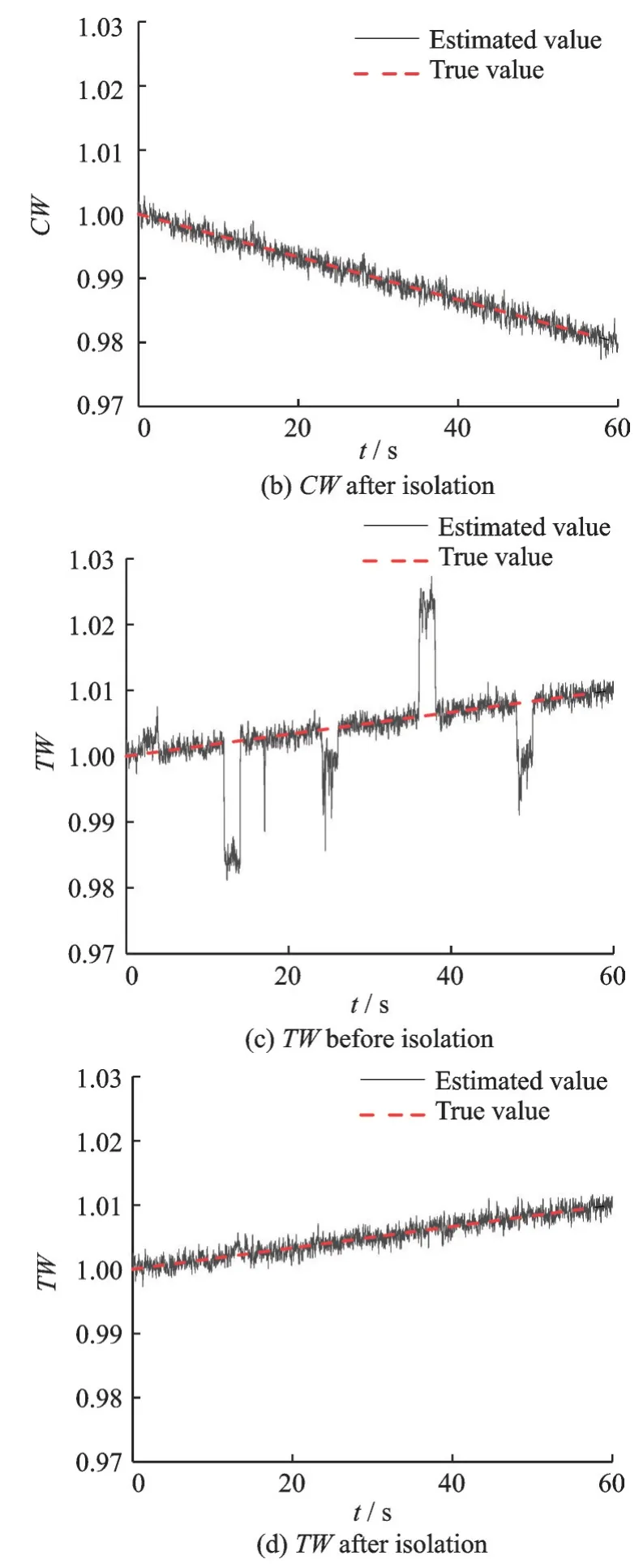
Fig.14 Flow capacity coefficient estimation in the case of single sensor fault with gradual degradation of gas path

From Figs.13 and 14，during the period in which sensor fault occurs，the estimated values of flow capacity coefficients before isolation have abrupt changes，so the flow capacity coefficients are not estimated correctly.After isolation，the recon⁃structed sensor value replaces the wrong one，so the estimated values of flow capacity coefficients are the same as those without sensor fault.The isolation distinguishes gas path degradation from sensor fault，and the isolation effect is good.

4.3.2 Dual sensor and component fault

In addition to the above sensor faults added in a dual-sensor fault situation，the gradual degradation mode of gas path is employed to the APU.The flow capacity coefficients estimation results before and after isolation are shown in Fig.15.

Fig.15 Flow capacity coefficient estimation in the case of dual sensor fault with gradual degradation of gas path

In the case of dual sensor fault，the estimated values of flow capacity coefficients before isolation have abrupt changes during the period in which the sensor fault occurs，so the flow capacity coefficients are not estimated correctly.After isolation，the flow capacity coefficients satisfy the linear variation law.

5 Conclusions

This paper has proposed an application of the DEKF algorithm combined with a packet loss mod⁃el on APU.The algorithm successfully estimates the flow capacity coefficients for gas path abrupt degradation and gas path gradual degradation in the situation of sensor faults.

In the steady condition，the fault detection and isolation of the five sensors are successfully realized under the distributed architecture by using the DEKF algorithm in single and dual-sensor fault con⁃ditions.When the gas path fault and sensor fault oc⁃cur simultaneously，the sensor isolation module ac⁃curately distinguishes gas path degradation from sen⁃sor fault.The sensor faults are eliminated timely and effectively，so the estimation of flow capacity coefficients is still accurate and not affected by the faulty sensors.