An elliptical blade is not a true ellipse,but a superellipse–Evidence from two Michelia species

Yuping Li · Karl J. Niklas · Johan Gielis ·Ülo Niinemets · Julian Schrader · Rong Wang ·Peijian Shi

Abstract The shape of leaf laminae exhibits considerable diversity and complexity that reflects adaptations to environmental factors such as ambient light and precipitation as well as phyletic legacy.Many leaves appear to be elliptical which may represent a ‘default’ developmental condition.However, whether their geometry truly conforms to the ellipse equation (EE), i.e., ( x/a) 2 + ( y/b) 2=1, remains conjectural.One alternative is described by the superellipse equation (SE), a generalized version of EE, i.e., | x/a| n +| y/b| n =1.To test the efficacy of EE versus SE to describe leaf geometry, the leaf shapes of two Michelia species (i.e., M.cavaleriei var.platypetala, and M.maudiae), were investigated using 60 leaves from each species.Analysis shows that the majority of leaves (118 out of 120) had adjusted root-mean-square errors of ＜ 0.05 for the nonlinear fitting of SE to leaf geometry, i.e., the mean absolute deviation from the polar point to leaf marginal points was smaller than 5% of the radius of a hypothesized circle with its area equaling leaf area.The estimates of n for the two species were ＜ 2, indicating that all sampled leaves conformed to SE and not to EE.This study confirms the existence of SE in leaves, linking this to its potential functional advantages,particularly the possible influence of leaf shape on hydraulic conductance.

Keywords Bilateral symmetry·Leaf ellipticalness index·Leaf laminae·Leaf roundness index ·Magnoliaceae

Introduction

In geometry, the ellipse is described by Eq.1 (denoted henceforth as EE for convenience):

wherexandyrepresent the abscissa and ordinate of the ellipse curve in the Euclidean plane, andaandb(≤a)represent the major and minor semi-axes, respectively.Whena=b, Eq.1 describes a circle.Lamé ( 1818) proposed a more general equation that is referred to as the superellipse equation (SE):

wherenis a positive real number that can be an integer or a non-integer (Gielis 2003a).Equation 2 uses an absolute value for bothx/aand fory/b, thereby making itsnpower meaningful for a negative value ofxory.Although SE has been applied to some artificial landscape and picture designs (e.g., a running track of an athletic field, and the profile of the new logo of Xiaomi, a Chinese multinational electronics company), there are still very few examples of the SE confirmed for natural geometries.Although many natural geometries are considered to be likely superellipses (Gielis 2003a), actual tests have not been performed,in part because of the limitations of data-fitting technologies.Shi et al.( 2015a) developed a practical technology for SE data-fitting, and fitted empirically determined tree-ring cross sections using SE.Their analysis confirmed that the cross sections of white spruce,Picea glauca(Moench) Voss,conformed to an SE, with estimates ofnranging from 1.7 to 2.3.Huang et al.( 2020) proposed an SE with a deformation parameter that described the cross sections of the stems of the square bamboo,Chimonobambusa utilis(Keng)Keng.The estimates ofnranged from 1.5 to 3.0 for ca.750 cross sections through 30 culms ofC.utilis.They also found that the outer rings of those cross sections had two types of superellipses: (1) a hyperellipse withn＞ 2 and, (2) a hypoellipse with 1 ＜n＜ 2.In these two studies, none of the cross sections were shown to be elliptical because the estimatedndeviated significantly from 2.These results highlight that some important natural geometries, appearing to be ellipses,are in fact superellipses.

The aforementioned biological studies have focused on the cross sections of stems.Thus, the question remains as to whether leaves that appear to be elliptical are in fact elliptical or are perhaps superelliptical.Leaves are the photosynthetic organs of the majority of vascular plants.Their diverse geometries, shapes, and sizes ref lect adaptations to mechanical, hydraulic, and other factors related to photosynthesis (Niklas 1992, 1999).For example, the venation patterns of the leaf lamina are correlated with leaf shape and geometry that collectively affect the sensitivity of hydraulic conductance to damage (Runions et al.2005;Scoffoni et al.2011), which is intimately associated with photosynthetic efficiency (Brodribb et al.2007).Thus, leaf shape plays a significant role in plant growth and survival.“Elliptical” leaf shapes commonly exist in most floras.However, no relevant studies have been carried out to test whether these geometries truly conform to the EE or to the SE equation.Considering that leaf geometry reflects the spatial distribution patterns of minor leaf veins (Niinemets et al.2007; Sack and Scoffoni 2013; Carvalho et al.2018), the analysis of leaf geometry in the context of EE vs.SE equivocality can improve our understanding of leaf hydraulic conductance and adaptive evolution.

In this study, the leaves of twoMichelia(Magnoliaceae)species, which appear to have elliptical geometries, were used to test and compare the validities of EE and SE in describing leaf geometry.

Materials and methods

Leaf sampling

Sixty mature, undamaged leaves were randomly collected from the middle canopies ofMichelia cavalerieivar.platypetala(denoted henceforth as MCP) andM.maudiae(denoted henceforth as MM) growing in the Nanjing Forestry University Campus (118°48′30′′ E, 32°4′49′′ N) on September 4, 2020 and September 13, 2020, respectively.The two species had been introduced from southern China where the species are naturally distributed.Four adjacent trees were selected for leaf sampling.Diameters at breast height ranged from 9.5 to 12.5 cm and heights from 5 to 6 m.The light conditions were comparatively high because the four trees were growing along a path that allows most parts of the crowns open to the sky.The ranges in diameters and heights were considered unimportant because there is no evidence that leaf geometry is affected or influenced by tree age nor is there evidence for any significant differences between shade and sun leaves forMicheliawith entire, nonserrated leaves without lobes.Therefore, leaf samples were taken from the trees without distinguishing between shade and sun leaves.

Leaves of theMicheliaspecies are well-suited for determining whether their elliptical geometries can be described by SE because they have been described as being elliptical.The laminae of these leaves are slightly axis-asymmetric with respect to the mid-vein, i.e., the lamina areas on each side of the mid-vein are unequal (Fig.1 A and B).

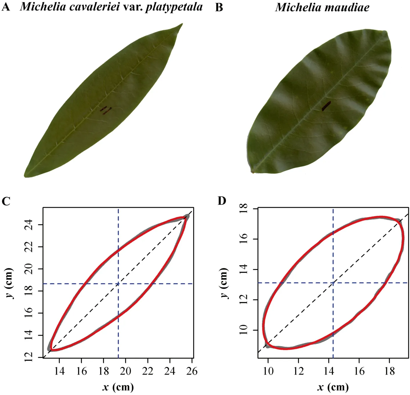
Fig.1 Examples of the leaves of two Michelia species and predicted leaf geometries based on the superellipse equation:M.cavaleriei var.platypetala( A and C); M.maudiae ( B and D).In panels C and D, the gray curves represent the actual(scanned) geometry, whereas the red curves represent the predicted geometry using the superellipse equation; the black dashed line represents the major axis

Data analysis

Leaf roundness index (RI) (Niinemets 1998; Peppe et al.2011) and leaf ellipticalness index (EI) (Li et al.2021) were used to measure the extent to which lamina geometry deviated from a circle or an ellipse using Eqs.3 and 4:

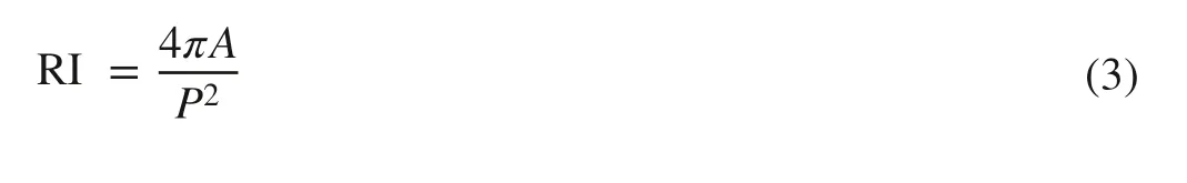
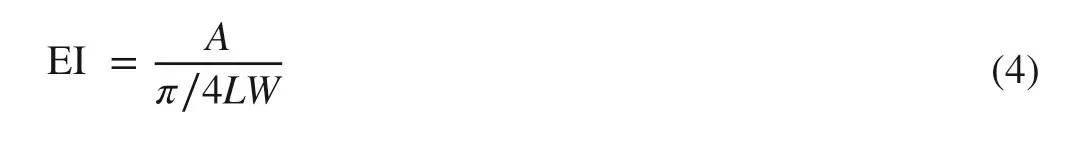
whereAis lamina area,Pis lamina perimeter,Lis lamina length, andWis lamina width.It is necessary to point out that the use of EI is limited to oval and elliptical leaves with values ranging from 0 to 1 and should not be used to assess leaves with values ＞ 1 (Li et al.2021).The numerical values ofA,P,LandWwere obtained from the planar coordinates of lamina edges using the R script developed by Su et al.( 2019).

In order to reduce the parameter-effects curvature in non-linear fitting, the re-parameterized version of SE(i.e., Eq.2) was used in the polar coordinate system (Ratkowsky 1990; Shi et al.2015a; Huang et al.2020; Tian et al.2020):

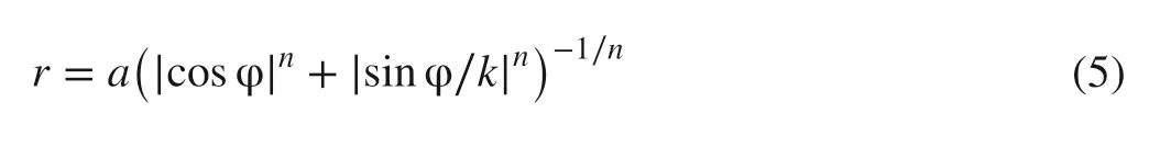
whereris the polar radius, φ is the polar angle,x=rcosφ,y=rsinφ, andk=b/a, whereaandbare the major and minor semi-axes, respectively.In the range of 0 to 2π, the residual sum of squares (RSS) was minimized between the actual and predicted polar radii of SE to estimate the parameters of SE.It should be noted that the coordinates of the polar point and the angle between the scanned major axis and thex-axis are unknown and must be estimated computationally.In addition to the three leaf-shape parametersa,kandn, there are three location parameters, i.e., thex- andy-coordinates of the polar point, and the rotation angle (for details see Shi et al.2015a).In order to measure the goodness of fit of the nonlinear regression, the adjusted root-mean-square error(RMSEadj) was used (Wei et al.2019; Huang et al.2020;Shi et al.2020):

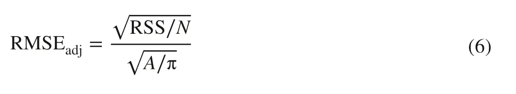
whereNrepresents the sample size, i.e., the number of data points on a leaf edge.The RI, EI, RMSEadjandnvalues between the two species were compared using the Tukey’s honestly significant difference (HSD; Hsu 1996).Note that,if leaf geometry conforms to the SE, leafAis theoretically proportional to the product of leafLandW(Huang et al.2020; Weisstein 2021):

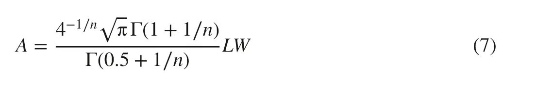
where Γ(·) is the gamma function.Thus, the following equation is obtained where,cis a constant to be fitted.Note that Eq.8 is referred to as the Montgomery equation, and the proportionality coefficient is the Montgomery parameter (Montgomery 1911;Shi et al.2019, 2021; Yu et al.2020; Schrader et al.2021).

In order to stabilize the variance of leafAin a linear regression, both sides of Eq.8 were log-transformed:

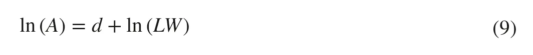
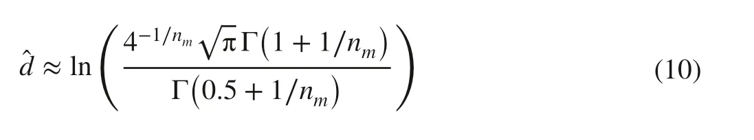
whered= ln(c).Ordinary least-squares regression protocols were used to fit Eq.9 with a slope equal to one.The bootstrap percentile method was used to compare whether there was a significant difference in the estimated Montgomery parameters between the two species (Efron and Tibshirani 1993; Sandhu et al.2011).Finally, if leaf geometry follows SE, it is possible to compare the intercept of Eq.9 with the natural logarithm of the proportionality coefficient of Eq.7 calculated from the median of the estimatednvalues for individual leaves (n m), i.e.,

All data analyses were carried out in R (v.4.0.2; R Core Team 2020).

Results

The leaf geometry of the twoMicheliaspecies deviated from that of a circle and tended toward an ellipse.The leaf roundness index (RI) and ellipticalness index (EI) of MCP were significantly smaller than those of MM (Fig.2 A, B).For both species, EI was greater than RI, indicating that the two leaf geometries were more likely to be ellipses (withn≠ 2 in the light of the inequality of leaf length and width)than circles.Thus, both leaf geometries could be evaluated to determine whether the superellipse equation (SE) or the ellipse equation (EE) provided a better fit.

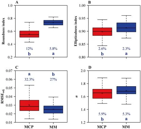
Fig.2 Comparisons of the leaf roundness indices A leaf ellipticalness indices B adjusted root-mean-square errors C and estimates of n D between the two Michelia species; the letters indicate the significance of the difference, and a and b represent larger to lower mean; the percentage numbers represent the coefficients of variation for the two species; MCP: M.cavaleriei var.platypetala;MM: M.maudiae

Subsequent analyses indicated that SE described the leaf geometry of both species.The adjusted RMSE values for the majority of leaves (118/120) were smaller than 0.05 (Fig.2 C), indicating that the mean absolute deviation between the actual and the predicted radii did not exceed 5% of the radius of the hypothesized circle whose area was equal to leaf area.All estimates ofnwere smaller than 2,confirming that the leaf geometries of MCP and MM conformed to the predictions of SE rather than EE and that the leaf geometries were hypoellipses.Figure 1 C, D show the fitted hypoellipse curves for two representative leaves.

95% CIs represent the 95% confidence intervals of the Montgomery parameter.Panels (A-B) show the fitted results of the two species,and panel (C) shows the combined data from the two species; in each panel, small open circles represent the data ofAvs.LWon a log–log scale, and the red regression line with slope=1 is based on ordinary least-squares regression

The fitted results of the Montgomery equation to the data of ln (A) vs.ln (LW) further confirmed the applicability of SE.The calculated intercept based on the median of the estimatednvalues using Eq.10 was approximately equal to that based on the linear regression for both species as well as the pooled data for the two species (Fig.3).Although the RMSE2value based on the median of the estimatednvalues was slightly greater than that of RMSE1based on the linear regression, all RMSE2values were numerically smaller than 0.05 (Fig.3).The estimated Montgomery parameter of MM was significantly greater than that of MCP based on the upper limit of the 95% confidence intervals of the difference of bootstrap replications between MCP and MM, which was smaller than 0 (Fig.4).

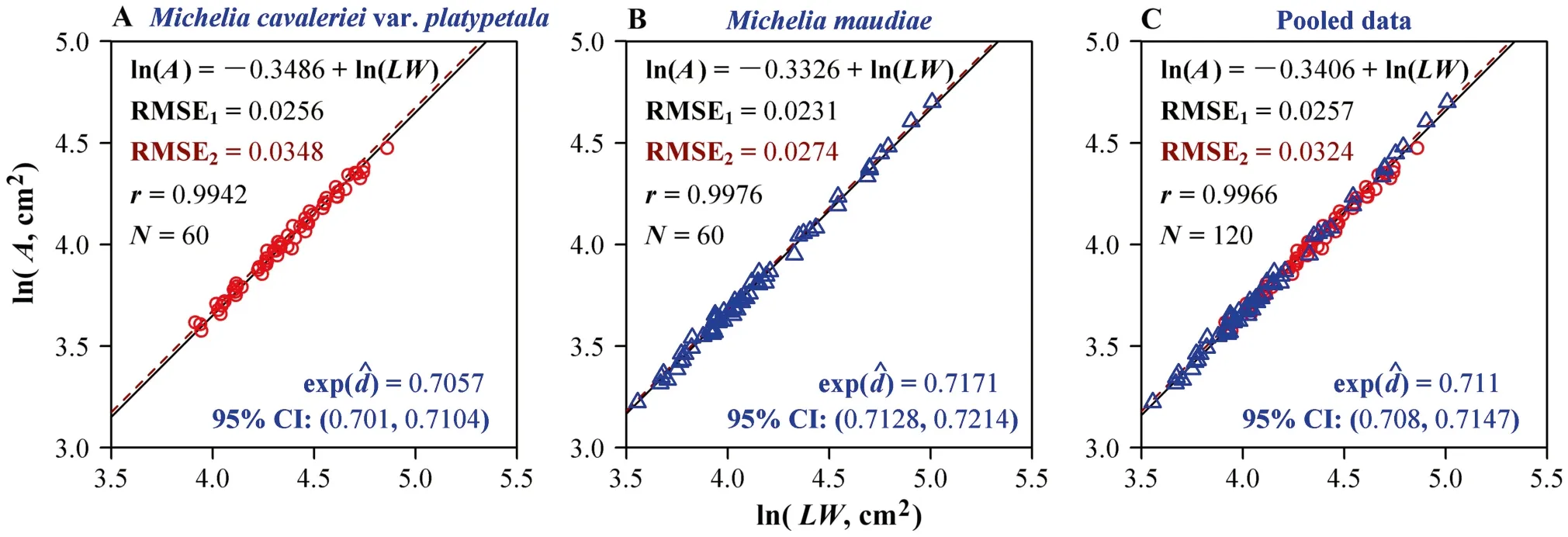
Fig.3 Fitted results of the Montgomery equation to the data from the two species for leaf area ( A) vs.the product of leaf length ( L) and width ( W) on a log–log scale.RMSE 1 is the root-mean-square error of the linear regression; RMSE 2 is the root-mean-square error based on the median of the estimated n values using Eq.10; r is the correlation coefficient of the regression of A vs.LW on a log–log scale; N is sample size; exp ( ^d ) is the estimated Montgomery parameter; the

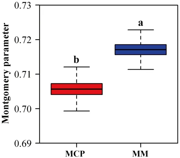
Fig.4 Comparison of the estimated Montgomery parameters for the two Michelia species (MCP vs.MM).The mean Montgomery parameter of MM is significantly greater than that of MCP (indicated by a ＞ b).The boxplots represent the 4000 bootstrap replications for each dataset.MCP: M.cavaleriei var.platypetala; MM: M.maudiae

Discussion

The objective of this research was to determine whether the leaf geometries of twoMicheliaspecies could be regarded as ellipses or superellipses withn≠ 2, using the conformity of the data to compare the ellipse equation (EE) and the superellipse equation (SE).The analyses show that the SE,which can only produce centrosymmetric geometries, categorically describes the leaf geometries of both species to a better degree than the EE.

Prior studies of the geometries of tree rings (best described as cross sections through tree growth layers) of conifers and the stems of bamboo indicate thatn-values range between ＞ 2 and ＜ 2 (Shi et al.2015a; Huang et al.2020), i.e., the cross-sectional geometries of these stems are hyperellipses or hypoellipses, and not ellipses.In this study,our data reveal thatn＜ 2 for bothMicheliaspecies.Thus, the leaf geometries of these two species are specifically hypoellipses.This result should not be taken as evidence that all“elliptical” leaves are hypoellipses.This aspect of leaf morphometry requires extensive additional research on a species by species basis.

In fact, the geometries of angiosperm leaves are extremely diverse, which prompted Gielis ( 2003b) to put forth a generalized Lamé curve with an equation in the polar coordinate system:

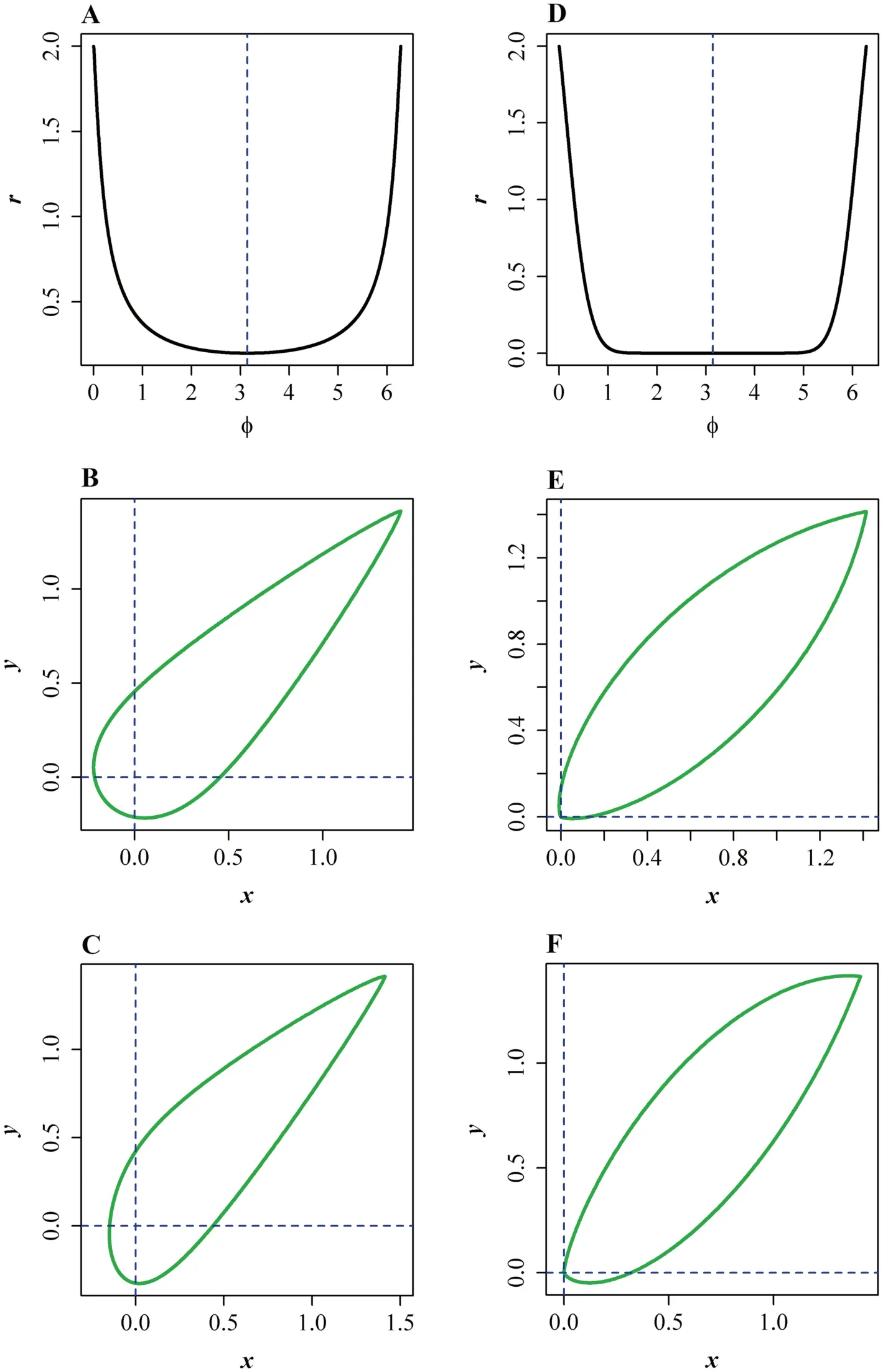
Fig.5 Relationships among the polar radius ( r) and polar angle (φ) and simulated leaf geometries.A Eq.13 with a = 2,b = 0.2 and n = 1.2; B the leaf geometry generated by Eq.13 without a deformation parameter; C the leaf geometry generated by Eq.13 with a deformation parameter=0.7; D Eq.15 with α=1.5, β=2.5 and γ=2;E the leaf geometry generated by Eq.15 without a deformation parameter; F the leaf geometry generated by Eq.15 with a deformation parameter=0.7.The deformation parameter is the same as that defined by Huang et al.( 2020)

wheremis a positive integer determining the number of angles of the curve in the range of 0 to 2π, andn1,n2, andn3are constants to be fitted.Shi et al.( 2015b, 2018) proposed a simplified version of the original Gielis equation:

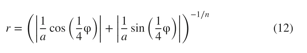
which describes the leaf geometries of bamboo species (Shi et al.2015b, 2018; Lin et al.2016).Here, another simplified Gielis equation is proposed:

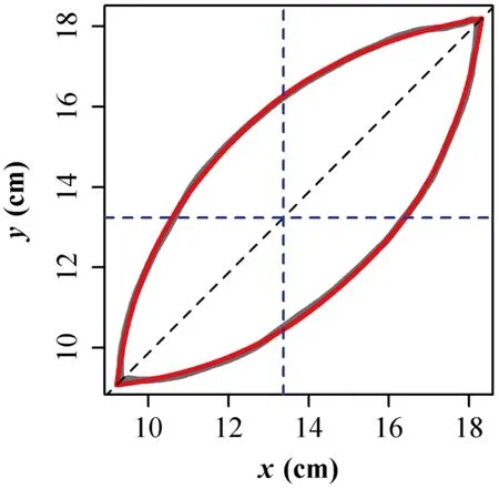
Fig.6 A representative leaf of Michelia cavaleriei var.platypetala and the predicted leaf geometry based on Eq.15.The gray curve represents the actual scanned leaf, whereas the red curve represents the predicted leaf geometry using Eq.15; the black dashed line represents the major axis.The raw planar coordinates of the leaf edge can be found in the online supplementary Table S1 corresponding to the code 1–30.The adjusted RMSE equals 0.0144, which means that the average absolute deviation of the curve fitting is less than 1.5% of the radius of a circle assuming that its area is equal to the leaf area.

which is a special case of the original Gielis equation(Eq.11) whenm= 2 andn1=n2=n3.Figure 5 A - C provide an example of this curve shape.Equation 13 can generate ovate geometries similar to those generated by Eq.12 and it is more flexible owing to an additional parameter.Equation 11 was proposed originally as a transformation on classical planar curves such as circles, ellipses, rectangles,superellipses and logarithmic spirals.It has a form similar to that of Eq.13.By replacingm= 2 withm= 5, Eq.13 has been used as a transformation on Grandi curves to model flowers (Gielis et al.2020).However, it still cannot generate the slight asymmetry between the leaf base and leaf tip that is evident in the leaves of the two species used in this study(and that is seen across leaves of many other species).This aspect of Eq.13 is possibly a consequence of the intrinsic limitations of trigonometric functions.Thus, it is more appropriate to consider the following more general function:

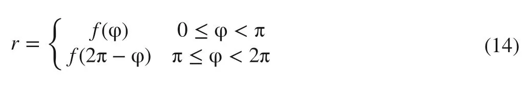
wheref(·) is a parametric function.This equation can produce any arbitrary curve determined by theffunction.Therefore, any bilateral symmetric leaf geometry can be theoretically parameterized and described, provided that a suitableffunction can be isolated to depict one-side of each leaf lamina (from 0 to π).To this end, we propose an exponential parabolic function:

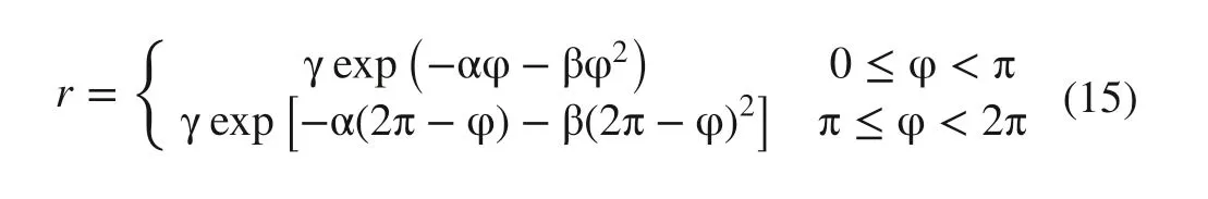
where α, β and γ are constants to be fitted.Figure 5 D - F provide an example of the utility of Eq.15, and show that this equation can produce a slight acropetal to basipetal asymmetry.The deformation matrix proposed by Huang et al.( 2020) can be used to explain such a deviation from a perfect bilateral symmetry along the leaf length axis.Figure 5 C, F provide two deformed examples.Figure 6 illustrates the validity of this approach in describing the actual leaf geometry ofM.cavalerieivar.platypetala.However,it is premature to suggest that Eq.15 is better than Eq.11.What can be asserted is that Eq.15 has the potential to be significantly useful in describing leaf geometry.

Importantly, Eqs.12 and 13 exceed the morphometric scope of SE, and each of these equations can be regarded as a special case of the original Gielis equation (i.e., Eq.11).Equation 14 is a generalized form of Eqs.11 and 15.Clearly however,extensive research is required to test the suitability of these equations to describe organic forms such as the geometries of leaves and stem cross sections.

Conclusions

The geometries ofM.cavalerieivar.platypetalaandM.maudiaeleaves are adequately described by the superellipse equation (SE), although there remains some degree of deviation from the axis-asymmetry between the leaf base and the leaf tip.The adjusted root-mean-square errors(between the actual and predicted polar radii) for most leaves (118 out of 120) are smaller than 0.05, indicating that the mean absolute deviation is less than 5% of the radius of a circle whose area is hypothesized to be equal to leaf area.The estimates ofn, an important parameter of the SE, range from 1.4 to 1.9 and therefore are smaller than 2.0 for each of the two species.This result indicates that leaf geometries of both species are hypoellipses.This study is the first to show that leaf geometry can be adequately described using the superellipse equation.Consequently, the description of leaves as “elliptical” may be in error in many cases (some may be superelliptical in geometry).This allegation requires future research into the morphometric description of leaf geometries, and may contribute to the development of models of leaf development and to the evolution ofimportant functional traits relating geometry to hydraulic and mechanical aspects affecting photosynthesis.

Open AccessThis article is licensed under a Creative Commons Attribution 4.0 International License, which permits use, sharing, adaptation, distribution and reproduction in any medium or format, as long as you give appropriate credit to the original author(s) and the source,provide a link to the Creative Commons licence, and indicate if changes were made.The images or other third party material in this article are included in the article’s Creative Commons licence, unless indicated otherwise in a credit line to the material.If material is not included in the article’s Creative Commons licence and your intended use is not permitted by statutory regulation or exceeds the permitted use, you will need to obtain permission directly from the copyright holder.To view a copy of this licence, visit http:// creat iveco mmons.org/ licen ses/ by/4.0/.