Analytical formula describing the non-saturating linear magnetoresistance in inhomogeneous conductors

Shan-Shan Chen(陈珊珊), Yang Yang(杨阳), and Fan Yang(杨帆)

Center for Joint Quantum Studies and Department of Physics,School of Science,Tianjin University,Tianjin 300350,China

Keywords: linear magnetoresistance,effective medium theory

1. Introduction

The magnetoresistance(MR)of a conventional conductor usually increases quadratically with magnetic fieldBat low fields and saturates at high fields. However, in the last few decades, a non-saturating linear magnetoresistance (LMR)has been observed in a wide variety of materials, including narrow-gap semiconductors,[1–3]graphene,[4–8]topological insulators,[9,10]topological semimetals,[11–14]and materials with charge-density-wave or spin-density-wave order.[15–19]In contrast to the conventional MR, the LMR observed in these materials exhibits a non-saturating quadratic-to-linear field dependence: As magnetic fieldBincreases,the function form of MR curves gradually changes from ∆ρ/ρ0∼B2to ∆ρ/ρ0∼Band the linearBdependence keeps up to very high fields.

Several theories have been developed to explain the nonsaturating LMR. These theories can be generally classified into two categories. The first category are quantum theories which take account of specific quantum mechanical processes of electrons,such as the condensation of electrons into the lowest Landau level[20,21]or the electron scattering at the hot spots of the Fermi surface due to charge-density-wave fluctuations.[15]The second category includes semiclassical theories which attribute the LMR to inhomogeneous distributions of carrier density or mobility in the sample.[22–27]Although quantum LMR has been experimentally reported in a few material systems,[3,5,15,16]the LMR observed in most materials were considered to be disorder-induced LMR which can be well understood within the framework of semiclassical theories.[3,4,6–10,19]

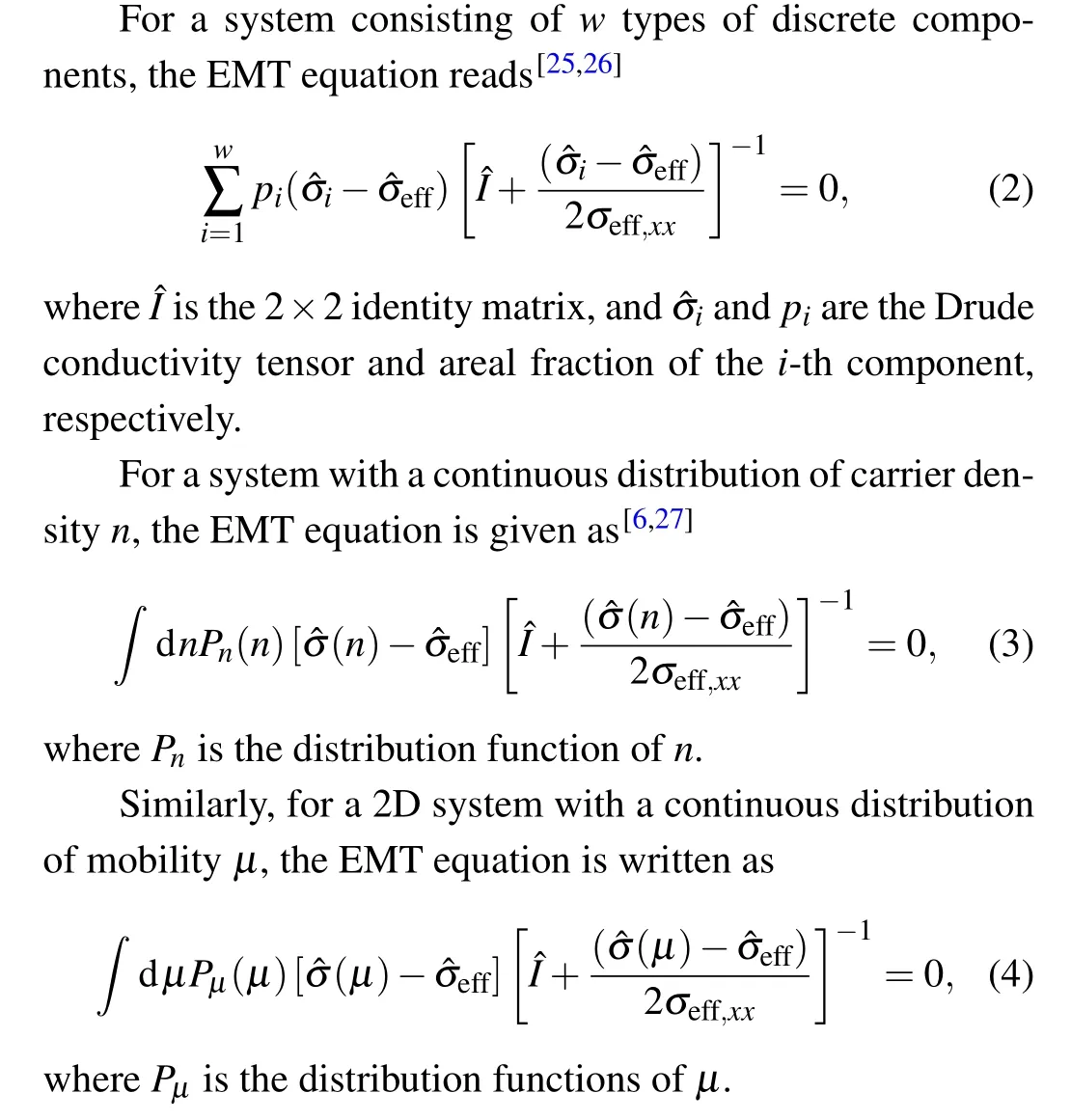
As one of the most successful semiclassical theories of disorder-induced LMR, the effective-medium theory (EMT)was first introduced by Stroud and Pan in 1975 to calculate the effective conductivity of an inhomogeneous system.[25]In 2005, Guttal and Stroud derived the EMT equations for two-dimensional (2D) systems consisting of two different components.[26]When the areal fractions of the two ingredients are equal, the two-componet EMT equations predict a non-saturating LMR very similar to the one observed in silver chalcogenides.[1,2,26]Soon after,the two-component EMT was employed to explain the MR of graphene near the Dirac point and satisfactory results were obtained.[28,29]In 2014,Pinget al.derived the EMT equations for disordered systems with a continuous distribution of carrier densityn.[6]The predictions of the continuous EMT were found to be quantitatively consistent with the experimental data obtained in graphene.[6]

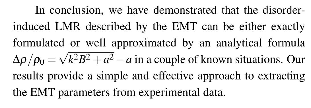
Although the EMT has proved successful in modeling the LMR of disordered systems, in practice, it is still difficult to directly compare the predictions of the EMT with experimental data, because calculating MR curves using the continuous EMT requires solving coupled integral equations which have no analytical solutions.In this paper,we propose that the LMR curves predicted by the EMT can be either exactly expressed or well approximated by an unified analytical formula

wherekandaare two phenomenological parameters usually determined by curve fitting. The relations between the EMT parameters and the phenomenological parameterskandaare evaluated. Our results provide a convenient and effective tool for analyzing the LMR data with the EMT.

2. Theoretical methods

2.1. Effective medium theory

The Drude resistivity tensor ˆρ(r) of an inhomogeneous conductor varies with positionrand thus cannot be measured experimentally by conventional methods. In this case,the results of resistivity measurements actually correspond to the elements of the effective resistivity tensor ˆρeffwhich is defined by〈E〉= ˆρeff〈J〉,whereEandJare electric field and current density, respectively. Here the angle brackets denote volume average,the same hereinafter. Similarly,the effective conductivity tensor ˆσeffis given by ˆσeff= ˆρ−1eff,which follows〈J〉= ˆσeff〈E〉.

The aim of the EMT is to calculate ˆσeffand ˆρeffby the mothed of mean-field approximation. In the approach of the EMT, an inhomogeneous system is considered to be locally homogenous,and each local region is treated as a circular area embedded in an effective medium with conductivity ˆσeff,which can be calculated self-consistently using the EMT equation.[25,26]The EMT equations for three different types of inhomogeneous 2D systems are listed in the following.

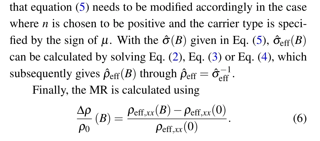
2.2. Calculation of magnetoresistance

2.3. Empirical equation for linear magnetoresistance

Equation (1) is an empirical equation for the LMR. It describes LMR curves which have a quadraticBdependence near zero field and a linearBdependence in high fields.

At the low-field limit (B →0), equation (1) reduces to∆ρ/ρ ≈(k2/2a)B2,while it approaches ∆ρ/ρ ≈kB−aat the high-field limit (B →∞). Therefore, the low-field quadratic coefficient(k2/2a)and the high-field slopekof LMR curves can be easily extracted by curve fitting using Eq. (1). In the following section, we will show that the LMR curves calculated from the EMT equations can be either exactly formulated or well fitted using the empirical equation given by Eq. (1).This finding will greatly facilitate the data analysis process of disorder-induced LMR.

3. Results and discussion

3.1. Systems consisting of two equally distributed components

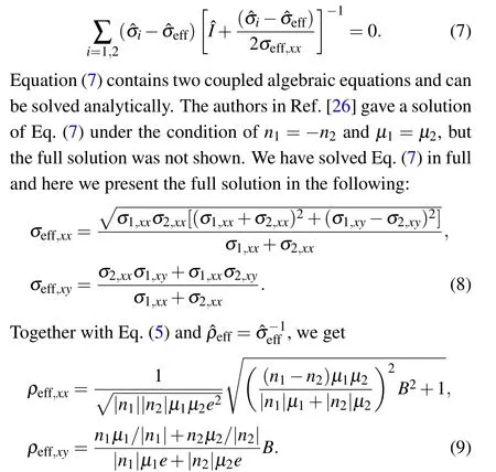
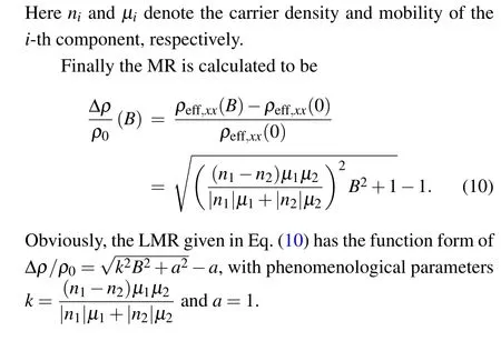
As discussed in Ref. [26], a 2D system consisting of two discrete components exhibits a non-saturating LMR only when the areal fractions of the two components are equal. In the following, we will prove that the LMR of such a system has exactly the function form of Eq.(1).

Withw=2 andp1=p2,equation(2)is simplified to

3.2. Systems with Gaussian distribution of n

In 2014, Pinget al.proposed a continuous model to explain the LMR in graphene.[6]In this model,the distribution ofnis taken to be a Gaussian functionPn=e−(n−〈n〉)2/∆n2,where〈n〉and ∆ndenote the average value and standard deviation ofn, respectively. In this case, the EMT equation of the system is given as

As discussed in Ref. [27], when plotted as a function of the dimensionless magnetic fieldµB, the LMR curves calculated from Eq.(11)depend only on the relative deviation of carrier density,i.e.,∆n/〈n〉.

As shown in Fig. 1(a), we have numerically calculated the LMR curves using Eq.(11)with various values of ∆n/〈n〉and fitted them using Eq. (1). The fitting results are reasonably good in the entire range ofµB,which indicates that equation (1) works very well as an empirical equation. The obtained parametersk/µandaare plotted as a function ofµBas shown in Fig. 1(b). As ∆n/〈n〉increases, the high-field slopek/µfirst increases rapidly and then gradually saturates at around ∆n/〈n〉=6.

Fig. 1. (a) Normalized magnetoresistance ∆ρ/ρ0 calculated using Eq. (11)with various ∆n/〈n〉, plotted against the dimensionless magnetic fieldµB. Dashed lines show the fits to the empirical equation ∆ρ/ρ0 =−a. (b) Fitting parameters k and a as a function of∆n/〈n〉,obtained from the empirical fitting shown in panel(a).

3.3. Systems with Gaussian distribution ofµ

Non-saturating LMR can also be realized in inhomogeneous systems with a Gaussian distribution ofµwhen〈µ〉=0,as discussed in Refs.[22,23]using the random-resistor model.Here we reproduce the LMR with the EMT and then demonstrate that the obtained LMR curves can be well fitted using Eq.(1).

LMR curves are obtained by numerically solving Eq.(12)with various values of ∆µ,as plotted in Fig.2(a). In this case,the obtained LMR curves are independent ofnbecausenis canceled out in the step of calculating ∆ρ/ρ0using Eq.(10). Fitting Eq.(1)to the LMR curves gives satisfactory results in the full range ofB,proving the validity of Eq.(1)as an empirical formula.

Fig. 2. (a) Normalized magnetoresistance ∆ρ/ρ0 calculated using Eq. (12)withvarious ∆µ. Dashed lines show the ftis totheempirical equation∆ρ/ρ0=k2B2+a2 −a. (b) Fittingparameterskandaas a function of∆µ,obtained from the empirical ftiting shown in panel(a).

The fitting parameterskandawere found to followk ≈0.4∆µanda ≈0.5626 in the entire investigated range of∆µ,as shown in Fig.2(b). Such a linear relationship betweenkand ∆µis consistent with previous results obtained using the random-resistor model.[22,23]In this situation, equation (1) is rewritten as

equation(13)can be directly used as an empirical equation for analyzing the LMR data of systems with a continuous distribution ofµ.

3.4. Further discussions

As shown in Figs. 1(b) and 2(b), the phenomenological parameterskandatake different values for the LMR curves originated from fluctuations ofnorµ. Therefore, these two situations can be easily distinguished by fitting Eq. (1) to the LMR data.

4. Conclusion

Acknowledgments

Project supported by the National Natural Science Foundation of China(Grant No.11904259)and the Natural Science Foundation of Tianjin(Grant No.20JC-QNJC02040).