Modified Subgradient Extragradient Method for Pseudomonotone Variational Inequalities

Jiajia Cheng and Hongwei Liu

(School of Mathematics and Statistics, Xidian University, Xi’an 710126, China)

Abstract: Many approaches have been put forward to resolve the variational inequality problem. The subgradient extragradient method is one of the most effective. This paper proposes a modified subgradient extragradient method about classical variational inequality in a real Hilbert interspace. By analyzing the operator’s partial message, the proposed method designs a non-monotonic step length strategy which requires no line search and is independent of the value of Lipschitz constant, and is extended to solve the problem of pseudomonotone variational inequality. Meanwhile, the method requires merely one map value and a projective transformation to the practicable set at every iteration. In addition, without knowing the Lipschitz constant for interrelated mapping, weak convergence is given and R-linear convergence rate is established concerning algorithm. Several numerical results further illustrate that the method is superior to other algorithms.

Keywords: variational inequality; subgradient extragradient method; non-monotonic stepsize strategy; pseudomonotone mapping

0 Introduction

For real Hilbert spaceHpossessing transvection 〈·,·〉 and norm ‖·‖, strong and weak converge of succession {xn} to a dotxare distinguished and expressed asxn→xandxn⇀x. With regard to a preset non-null, closed convex setC⊆H, variational inequality problem (VI (P)) need to be considered. A dotx′∈Cis sought and the below formula holds:

〈x-x′,F(x′)〉≥0,∀x∈C

(1)

As is known,x′is a solution of inequality (1) which equalsx′=PC(x′-λF(x′)) for allλ>0.

Variational inequality is a particularly practical model. Quite a few problems can be expressed as VI (P), for instance, nonlinear equation, complementarity matters, barrier questions, and many others[1-2]. In recent decades, some projection algorithms to solve VI (P) have been raised and developed by many researchers[3-11].

The most classical algorithm is projection gradient method[12-13]:

xn+1=PC(xn-λF(xn))

Only when the mappedFis a(n) (inverse) strong monotone L-Lipschitz consecutive mapping and the step length satisfiesλ∈(0,(2η)/L2), the convergence of algorithm can be obtained, whereL>0 andη>0 represent Lipschitz and strong monotonicity constants, respectively. To solve the monotone L-Lipschitz continuous variational inequality, Korpelevich[14]proposed an extragradient algorithm. This method has attracted the attention of many researchers and presents a variety of improved methods[15-19]. Later, Censor et al.[5]introduced an algorithm: the second projection is converted fromCto a specific semi-space, which is called subgradient extragradient algorithm. Its form is listed as follows:

zn+1=PTn(zn-λFxn),xn+1=PC(zn+1-λFzn+1)

where

The other part of this article is arranged as follows. Section 1 reviews several relevant knowledge topics for later use. Section 2 states a subgradient extragradient method with a non-monotonic stepsize strategy. Section 3 includes two parts: the weak convergence and R-linearly convergence rate under the hypothesis of pseudomonotonicity and strong pseudomonotonicity respectively. In the last section, two classical examples are given to explain the advantages of the proposed algorithm.

1 Preliminaries

Several notations and lemmas are provided for later use.

Definition1.1[22-23]For anyα,β∈H, assumeFonHis

(a) strongly monotone

∃γ>0,s.t.γ‖α-β‖2≤〈α-β,Fα-Fβ〉

(b) monotone

〈α-β,Fβ〉≤〈α-β,Fα〉

(c) strongly pseudomonotone

∃γ>0,s.t. 0≤〈β-α,Fα〉⟹

γ‖β-α‖2≤〈β-α,Fβ〉

(d) pseudomonotone

0≤〈α-β,Fβ〉⟹0≤〈α-β,Fα〉

(e) L-Lipschitz continuous

∃L>0,s.t. ‖Fα-Fβ‖≤L‖α-β‖

(f) sequentially weakly continuous: if random succession {αn} satisfiesαn⇀α, there isFαn⇀Fα.

Remark1[22]The deduced process of (a)⟹(b) and (c)⟹(d) are obvious. Furthermore, (a) and (c) ensure that VI (P) has at most one solution.

Lemma1.1[24]For a non-null closed convex setC⊆H, anyα∈H,β∈Csatisfies

(a)〈PCα-α,β-PCα〉≥0

(b)‖PCα-α‖2+‖PCα-β‖2≤‖α-β‖2

Lemma1.4[26]For VI (P),C⊆His a non-null enclosed convex andF:C→His pseudo-monotone successive.α′as an answer to VI (P) is equal to

〈α-α′,Fα〉≥0, ∀α∈C

Lemma1.5(Opial) Consider succession {αn}⊆H. Ifαn⇀αis true, there is

2 Algorithm

The proposed subgradient extragradient algorithm combines a non-monotonic stepsize strategy, which will be illustrated in this section.

AlgorithmA

Step1Take

x1=PC(x0-λ0F(y0)),y1=PC(x1-λ1F(y0))

Step2Knowing the present iteratesyn-1,xn, andyn, construct

Tn={x∈H:〈yn-x,xn-λnF(yn-1)-yn〉≥0}

and figure out

xn+1=PTn(xn-λnF(yn))

Step3Calculate a stepsize

λn+1=

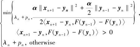
yn+1=PC(xn+1-λn+1F(yn))

Ifxn+1=xnandyn=yn-1( oryn+1=xn+1=yn), stop andynis a solution. Otherwise, letn∶=n+1, and go to Step 2.

ProofBecauseFis L-Lipschitz continuous mapping, if 〈xn+1-yn,F(yn-1)-F(yn)〉>0, then

which implies that

3 Convergence Analysis

The relevant convergence is given in this part. Firstly, some sequences weakly converging to the solution were analyzed and the R-linear convergence rate was obtained. Moreover, the following hypotheses is made about VI (P):

(A1) The disaggregationSof inequality (1) is non-null;

(A2)Fis pseudomonotone overHand weakly sequentially continuous overC;

(A3)Fis L-Lipschitz consecutive overH.

Convergence of the algorithm is discussed below. The following lemma is essential to gain the main theorem.

Lemma3.1Algorithm A can produce two successions {xn} and {yn}, which are bounded.

ProofForv∈S,yn∈Cnaturally has

〈yn-v,F(v)〉≥0, ∀n≥1

Then 〈yn-v,F(yn)〉≥0 in consideration of pseudomonotonicity, which in turn is equivalent to

〈yn-xn+1,F(yn)〉≥〈v-xn+1,F(yn)〉

(2)

The proving process is analogue to Lemma 3.3 of Ref. [23], it can be obtained that

2λn〈xn+1-yn,F(yn-1)-F(yn)〉

(3)

In accordance with the definition ofλn, inequality (3) yields that

(4)

N1>0 andG1>0, such that for anyn>N1, there is

Inequality (4) can be rewritten by

G1(‖yn-1-yn‖2+‖yn-xn+1‖2)

(5)

Forn>N1, set

By means of trigonometric inequality, there isxn→ynand {yn} is limited as well.

Theorem3.1Suppose that successions {xn} and {yn} are produced by Algorithm A, it can be deduced that they weakly converge to the same potx′∈S.

ProofLemma 3.1 yields the result that there is a sub-series {xnk}⊆{xn} that converges weakly to a dotx′.Obviously there is {ynk} weakly converging tox′∈C.

Sinceynk+1=PC(xnk+1-λnk+1F(ynk)), applying Lemma 1.1(a), there is

〈z-ynk+1,ynk+1-xnk+1+λnk+1F(ynk)〉≥0,∀z∈C

or equivalently

0≤〈z-ynk+1,ynk+1-xnk+1〉+λnk+1〈z-ynk+1,F(ynk)〉=〈z-ynk+1,ynk+1-xnk+1〉+λnk+1〈z-ynk,F(ynk)〉+λnk+1〈ynk-ynk+1,F(ynk)〉 Takingk→∞ in the above-mentioned expression, sinceλnk+1>0, the following is derived:

(6)

There is a positive succession {εk}, which decreases and has a limit of zero. A rigorously increasing sequence of positive integers {Nk} can be found, thus the inequality below is obtained:

εk+〈z-ynj,F(ynj)〉≥0, ∀j≥Nk

(7)

In light of inequality (6), it can be concluded thatNkexists. In addition, for eachk, let

There is 〈F(yNk),wNk〉=1. It follows from inequality (7) that for eachk, there is

〈z+εkwNk-yNk,F(yNk)〉≥0

Furthermore,Fis pseudomonotone overH, so there is

〈z+εkwNk-yNk,F(z+εkwNk)〉≥0

which corresponds to

〈z+εkwNk-yNk,F(z)-F(z+εkwNk)〉-

εk〈wNk,F(z)〉≤〈z-yNk,F(z)〉

(8)

Invoking Lemma 1.4 yieldsx′∈S.

Finally, the conclusion that {xn} converges weakly tox′is gained. Suppose that it has at any rate two weak accumulation dotsx″∈Sandx′∈S. At this time, there isx″≠x′.Let the limit of {xni} bex″, from Lemma 1.5 the following can be known:

Subsequently, (A2) was replaced with (A2*) to prove that Algorithm A has R-linear convergence rate.

(A2*)Fis strongly pseudomonotone overH.

Theorem3.2If the supposition (A1), (A2*), and (A3) comes into existence, Algorithm A can produce succession {xn}.It can be derived that {xn} at least R-linearly strongly converges to the only resolutionuof inequality (1).

Proof〈yn-v,F(v)〉≥0,∀v∈Sis true. According to the hypothesis thatFis strongly pseudo-monotone, the following formula is true:

γ‖yn-v‖2≤〈yn-v,F(yn)〉

It could also be described as

γ‖yn-v‖2≤〈yn-xn+1,F(yn)〉-

〈v-xn+1,F(yn)〉

(9)

Therefore, invoking the regulation ofTnin the Algorithm A yields that

〈xn+1-yn,xn-λnF(yn)-yn〉≤

λn〈xn+1-yn,F(yn-1)-F(yn)〉

(10)

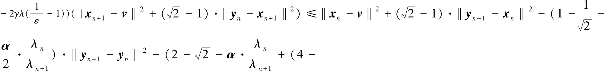
Combining Lemma 1.1 (b) and inequality (9) with inequality (10), the following can be derived:

‖xn+1-v‖2≤‖xn-v‖2-‖xn-xn+1‖2+2λn〈v-xn+1,F(yn)〉≤‖xn-v‖2-

‖xn+1-yn‖2-‖yn-xn‖2+2〈xn+1-yn,

xn-yn-λnF(yn)〉-2γλn‖yn-v‖2≤

‖xn-v‖2-‖xn-yn-1‖2-‖yn-1-yn‖2+2‖yn-1-yn‖‖xn-yn-1‖-‖yn-xn+1‖2+2λn〈xn+1-yn,F(yn-1)-F(yn)〉-2γλn‖yn-v‖2

(11)

(12)

From the form defined byλn, ∃N2>0,λ>0,∀n>N2s.t.λn>λ, ∀n>N2is obtained. The above formula can be arranged as

(13)

In short, denote

Invoking Lemma 1.2 can deduce

-‖yn-v‖2=-‖yn-xn+1‖2-‖xn+1-v‖2-2〈yn-xn+1,xn+1-v〉≤(ε-1)·

(14)

Using inequality (14), the following formula is obtained by rearranging inequality (13) and shifting items

(15)

Similar to the processing method in inequality (4), there isN3>N2>0,G2>0, such that for anyn>N3, there is

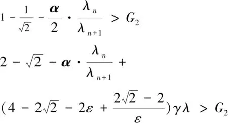
Then inequality (15) is equivalent to

(1+ρ)an+1≤an-bn,∀n>N3

From induction, it may be deduced that for ∀n>N3there is

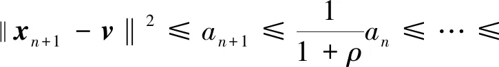
which completes the proof.

Remark2Compared with Theorem 2.1 in Ref. [23], the above theorem has three major advantages:

1) Fewer parameters are used;

2) A non-monotonic stepsize strategy is adopted instead of the monotonic decreasing stepsize;

3) The previous assumptions are weakened, namely,monotonicity are replaced with pseudomonotonicity and weak sequential continuity ofF, and strong monotonicity is replaced with strong pseudomonotonicity.

4 Numerical Results

By comparing Algorithm A with Algorithm 1[21]in numerical experiments, the effectiveness of the proposed algorithm is demonstrated.

The iteration times (ite.) and calculation time(t) conducted in all tests were recorded in seconds. The condition for terminating the algorithm was ‖xn+1-xn‖≤ε.For the tolerance,ε=10-6was set in all experiments. The following parameters were used in the algorithm mentioned below:

Table 1 Numerical results of Problem 1

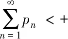
From Table 1,pncontrols the non-monotonicity of the stepsize. Whenpn=0, the stepsize decreases monotonically. At this time, the iteration will stop because the stepsize is too small to find the best point. Non-monotonic stepsize increases or decreases to quickly find the best advantage and make the iteration stop. It can also be seen that the non-monotone stepsize has less iterations and faster time than monotone stepsize.

Problem2The second question was applied to Refs. [28] and [29], where

H(x)=(h1(x),h2(x),...,hm(x))

2xi-1-1

x0=xm+1=0,i=1,2,...,m

As shown in Table 2, it can be observed that Algorithm A is more advanced than Algorithm 1 in terms of iterations and calculation time. Moreover, when the value ofαis larger, the effect of the new algorithm is better.

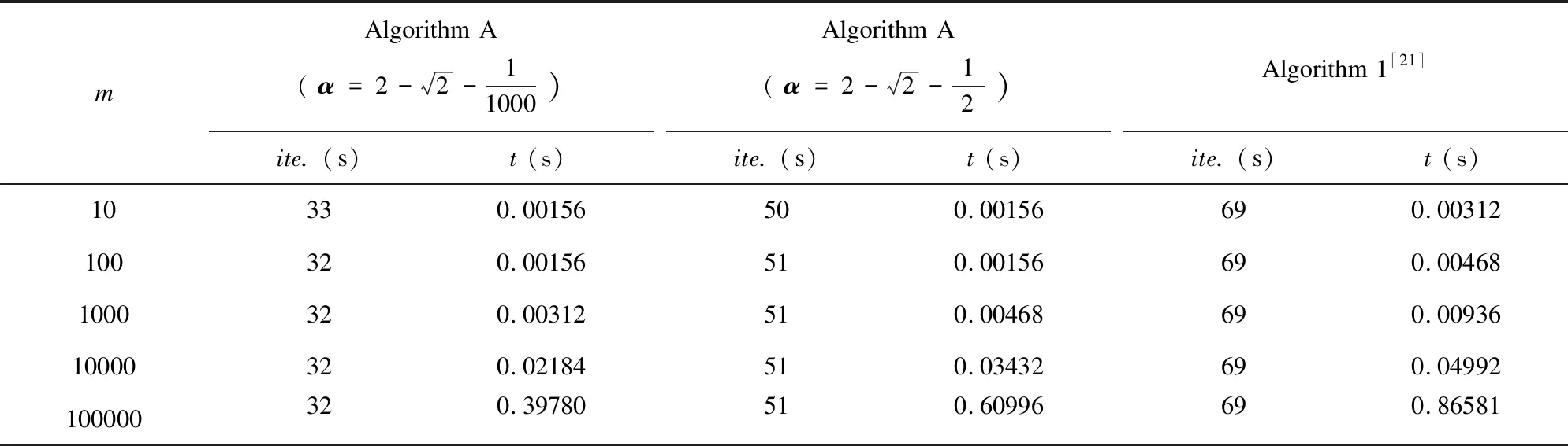
Table 2 Numerical results of Problem 2

5 Conclusions

The paper presents the convergence analysis of Lipschitz continuous pseudomonotone VI (P). When the value of Lipschitz constant is unclear, weak convergence of the sequence is proved by using non-monotonically updating stepsize strategy. Furthermore, the R-linear convergence rate of sequence was obtained and the performance of the scheme was demonstrated on some numerical examples to show the effectiveness of the proposed algorithms.