Robust Frequency Estimation Under Additive Mixture Noise

Yuan Chen, Yulu Tian, Dingfan Zhang, Longting Huangand Jingxin Xu

1School of Computer and Communication Engineering, University of Science & Technology Beijing,Beijing, 100083, China

2School of Automation Science and Electrical Engineering, Beihang University, Beijing, 100191, China

3School of Information Engineering, Wuhan University of Technology, Wuhan, 430070, China

4Department of Energy and Public Works, Queensland, 4702, Australia

Abstract: In many applications such as multiuser radar communications and astrophysical imaging processing, the encountered noise is usually described by the finite sum of α-stable (1≤α＜2) variables.In this paper, a new parameter estimator is developed, in the presence of this new heavy-tailed noise.Since the closed-form PDF of theα-stable variable does not exist except α= 1 and α= 2, we take the sum of the Cauchy (α= 1) and Gaussian(α= 2) noise as an example, namely, additive Cauchy-Gaussian (ACG)noise.The probability density function (PDF) of the mixed random variable,can be calculated by the convolution of the Cauchy’s PDF and Gaussian’s PDF.Because of the complicated integral in the PDF expression of the ACG noise, traditional estimators, e.g., maximum likelihood, are analytically not tractable.To obtain the optimal estimates, a new robust frequency estimator is devised by employing the Metropolis-Hastings (M-H) algorithm.Meanwhile, to guarantee the fast convergence of the M-H chain, a new proposal covariance criterion is also devised, where the batch of previous samples are utilized to iteratively update the proposal covariance in each sampling process.Computer simulations are carried out to indicate the superiority of the developed scheme, when compared with several conventional estimators and the Cramér-Rao lower bound.

Keywords: Frequency estimation; additive cauchy-gaussian noise; voigt profile; metropolis-hastings algorithm; cramér-rao lower bound

1 Introduction

Heavy-tailed noise is commonly encountered in a variety of area such as wireless communication and image processing [1-8].Typical models of impulsive noise are α-stable, Student’stand generalized Gaussian distributions [9-12], which cannot represent all kinds of the noise types in the real-world applications.Therefore, the mixture models have been developed including the Gaussian mixture and the Cauchy Gaussian mixture models [13,14], of which the probability density functions (PDFs) is the weighted sum of the corresponding components’PDF.However, these mixture models still cannot describe all impulsive noise types, especially for the case where the interference is caused by both channel and device.In astrophysical imaging processing [15], the observation noise is modelled as the sum of a symmetric α-stable (SαS) and a Gaussian noise, caused by the radiation from galaxies and the satellite antenna, respectively.Moreover, in a multiuser radar communication network [16], the multi-access interference and the environmental noise corresponds toSαSdistributed and Gaussian distributed variables.Therefore, a new description of the mixture impulsive noise model is proposed,referring to as the sum ofSαSand Gaussian random variables in time domain.

In this work, the frequency estimation is considered in the presence of the additive Cauchy-Gaussian (ACG) noise [17,18], which is the sum of two variables with one following Cauchy distribution (α= 1) [19] and the other being Gaussian process (α= 2).The PDF of ACG noise can be calculated by the convolution of the Gaussian and Cauchy PDFs.According to [20], the PDF of the mixture can be expressed as Voigt profile.Due to the involved form of the Voigt profile, classical frequency estimators [21-24], such as the maximum likelihood estimator (MLE) andM-estimator[25], has convergence problem and cannot provide the optimal estimation in the case of high noise power.To obtain the estimates accurately, Markov chain Monte Carlo (MCMC) [26-28] method is utilized, which samples unknown parameters from a simple proposal distribution instead of from the complicated posterior PDF directly.Among series of MCMC methods, the Metropolis-Hastings (MH) and Gibbs sampling algorithms are typical ones.The M-H algorithm provides a general sampling framework requiring the computations of an acceptance criterion to judge whether the samples come from the correct posterior or not.While in the case that the posterior PDF is easy to be sampled from, Gibbs sampling is utilized without the calculation of acceptance ratios.It is noted that once the posterior of parameters is known, M-H and Gibbs sampling methods can be utilized in any scenarios.

Because of the Voigt profile in the target PDF of the ACG noise, we choose the M-H algorithm as the sampling method.To improve the performance of the M-H algorithm, an updating criterion of proposal covariance is devised, with the use of the samples in a batch process.Since we assume all unknown parameters are independent, the proposal covariance is in fact a diagonal matrix.Therefore,the square of difference between the neighbor samples is employed as the diagonal elements of proposal covariance, referred to as the proposal variance.Meanwhile, a batch-mode method is utilized to make the proposal variance more accurate.As the proposal variance is updated only according to the samples in each iteration, this criterion can be extended to any other noise type such as the Gaussian and non-Gaussian processes.

The rest of this paper is organized as follows.We review the MCMC and M-H algorithm in Section 2.The main idea of the developed algorithm is provided in Section 3, where the PDF of the additive impulsive noise and posterior PDF of unknown parameters are also included.Then the Cramér-Rao lower bounds (CRLBs) of all unknown parameters are calculated in Section 4.Computer simulations in Section 5 are given to assess the performance of the proposed scheme.Finally, in Section 6, conclusions are drawn.Moreover, a list of symbols is shown in Tab.1, which are appeared in the following..

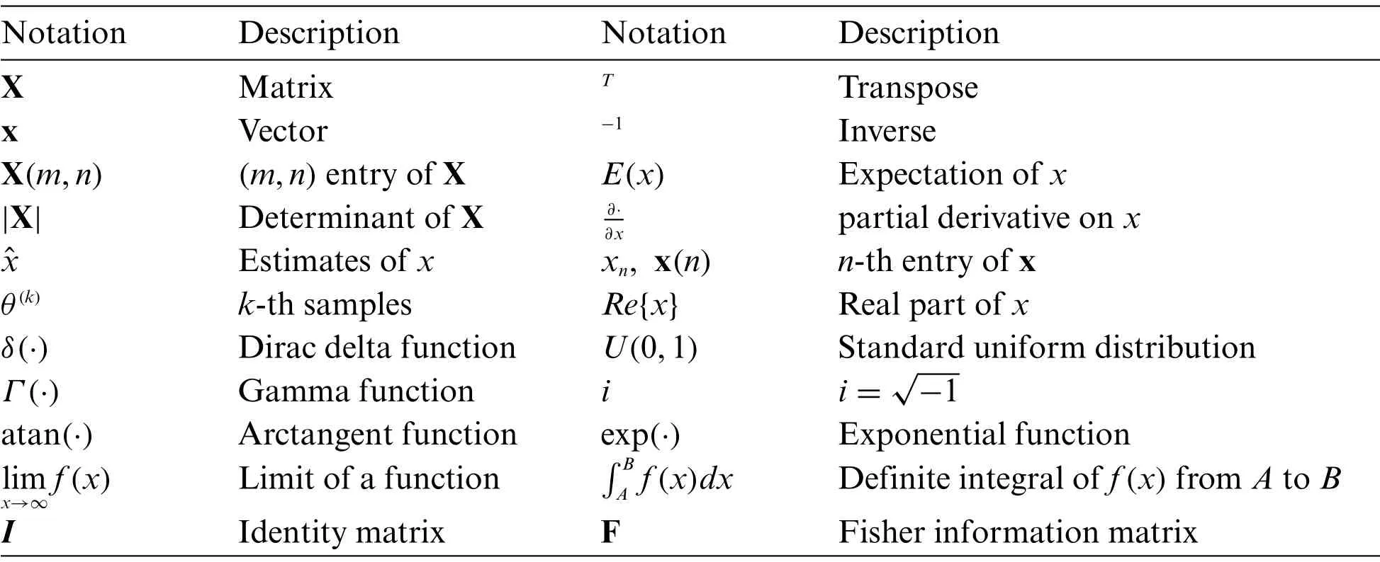
Table 1: List of symbols

2 Review of MCMC and M-H Algorithm

Before reviewing the M-H algorithm, some basic concepts, such as Markov chain should be introduced [29,30].By employing several dependent random variables {x(l)} [31], we define a Markov chain as

where the probability ofx(l+1)relies only on {x(l)} with the conditional PDF being defined by P(x(l+1)|x(l)).The PDF ofx(l+1), denoted by πl+1, can be expressed as

Then the Markov chain is said to be stable if

with π*=.To ensure (3), a sufficient but not necessary condition can be written as

Typical MCMC algorithms draw samples from the conditional PDF P(x(l+1)|x(l)) with a Markov chain, instead of directly sampling from a target PDFf(x).Therefore, if a proper conditional PDF P(·|·) is chosen, the stationary distribution can align with the target PDFf(x).In other word,samples drawn from a stable Markov chain will eventually tend to be generated fromf(x) accordingly.Furthermore, only samples generated from the stable Markov chain are independent and identically distributed (IID).

In the following, the details of the MCMC method are provided in Tab.2.It is worth to point out that the burn-in period is a term of an MCMC run before convergent to a stationary distribution.

Table 2: Steps of MCMC method

Among typical MCMC methods, M-H algorithm is commonly employed, whose main idea[32] is drawing samples from a proposal distribution with a rejection criterion, instead of sampling from P(x(l+1)|x(l)) directly.In this method, a candidate, denoted byx*is generated from a proposal distributionq(x*|x(l)).Then the acceptance probability is defined as

which determines whether the candidate is accepted or not.It is noted that the proposal distributions are usually chosen as uniform, Gaussian or Student’stprocesses, which are easier to be sampled.The details of the M-H algorithm can be seen in Tab.3.

Table 3: Steps of M-H algorithm

In the M-H algorithm, to prove the stationary, we define a transition kernel [33] as

where B(x(l)) =q(x*|x(l))(1 - A(x(l),x*))dx*.By employing (4), (6) can be rewritten as

Then we have

According to[33],it can be proven thatδ(x(l+1)-x(l))B(x(l))f(x(l)) =δ(x(l)-x(l+1))B(x(l+1))f(x(l+1)).Therefore, with the use of (8)-(9) as well as (4), the balance condition of the M-H algorithm can easily to be hold.

In this algorithm, samples obtained in each iteration are closing to each other and can be highly correlated since M-H moves tend to be local moves.Asymptotically, the samples drawn from the Markov chain are all unbiased and all come from the target distribution.

3 Proposed Method

Without loss of generality, the observed data y = [y1,y2,···,yN]Tis modeled as:

wherea1=Acos(φ),a2= -Asin(φ) withA,ω,φ denoting amplitude, frequency and phase, respectively.Theqn=cn+gnis the IID ACG noise, wherecnis the Cauchy noise with unknown median γ andgnis the zero-mean Gaussian distributed with unknown variance σ2.Here our task is estimatingA,ω and φ from observations.

3.1 Posterior of Unknown Parameters

Here we investigate the posterior of unknown parameters.Before that, we first express the PDFs of noise termscnandgnas:

Then the PDF of the mixture noiseqn, known as the Voigt profile [23], can be computed according to convolution of (9) and (10), which is

where

Let θ= [a1,a2,ω,γ,σ2]Tbeing unknown parameter vector.According to the investigation in [34],the unknown parametersa1anda2are usually assumed to be following the IID Gaussian distribution with variance δ2and zero mean.While ω is the continuous uniform distributed between 0 and π,respectively.

Furthermore, it is also assumed in [34] that both γ and σ2follows the conjugate inverse-gamma distributions.Therefore, the priors for all unknown parametersa1,a2,ω,γ and σ2can be written as

where α and β are set to α=10-10and β=0.01, respectively.

According to the PDF expression of ACG noise in (13), the conditional PDF of the observation vector y has the form of

whereen=yn-a1cos(ωn)-a2sin(ωn)denotes the residual between the observed data and the noise-free signal, and

Assume that the priors for all unknown parameters θ and the observations y are statistically independent.With use of (15)-(18) and (19)-(20) as well as Bayes’theorem [25], the posterior expression of all unknown parameters θ can be

3.2 Proposed M-H Algorithm

Due to themultimodality of the likelihood function, themaximumlikelihood estimator cannot beemployed and the high computational complexity of the grid search.Furthermore, other typical robust estimators, such as the ℓ1-norm minimizer [35], cannot provide optimum estimation for the mixture noise.Moreover, even when the posterior PDFs of each unknown parametersf(θ|y) are known, the Gibbs sampling algorithm cannot be applied because of the complicated expression in (21).

Therefore, to estimate parameters accurately, the M-H algorithm is utilized, whose details are provided in Tab.3.To simplify the sampling process, the multivariate Gaussian distribution is selected as the proposal distributionq(·|·).Inl-th sampling iteration,q(x*|x(l-1)) can be written as

where x*= [x1x2x3x4x5]Tis the candidate vector withx1,x2,x3,x4andx5corresponding toa1,a2,ω,γ and σ2, respectively,denotes the proposal mean vector with θ(l-1)being the samples in (l- 1) th iteration and the Σ(l)is the 5×5 proposal covariance matrix.With the assumption that all unknown parameters are independent, the Σ(l)is regarded as a diagonal matrix.Furthermore,the main diagonal entries of the proposalcovariance are also called the proposal variances.

It is noted that the larger proposal variance will cause a faster convergence but possible oscillation around the correct value.While the smaller values of proposal variance lead to slower convergence but small fluctuation.Therefore, the choice of the proposal variance will significantly influence the performance of the estimator.In this paper, a batch-mode proposal variance selection criterion is developed.

To estimate Σ(l),we define two new batch-mode vector using the formerLsamplingvectors,which are

whereLis also called the length of the batch-mode window.Then the proposal covariance Σ(l)can be defined by the empirical covariance of Φ1and Φ2, which is

To state the criterion clearly, the details are also shown in Fig.1.

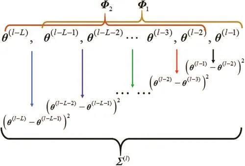
Figure 1: The construction of the proposal covariance

To start the algorithm, the initial estimate of θ and the burn-in periodPshould be determined.As it is discussed before,θ(1)can be chosen arbitrarily because the initialization of the M-H method only affects the convergence rate.To guarantee the enough samples in the batch-mode criterion,the firstPburn-in samples are generated with a fixed proposal covariance.From thel-th iteration(l=P+ 1,P+ 2,···),θ(l)is calculated by the M-Halgorithm using an adaptive Σ(l)..AfterKnumbers of sampling,the estimates,andare obtained fromthe mean of the first three row of the samples,which are

where θ(l)(1),θ(l)(2) and θ(l)(3) are the first three elements ofl-th sampling vector, respectively.The details of the proposed algorithm are shown in Tab.4.

Table 4: The proposed algorithm

Finally, utilize the definition ofa1=Acos(φ) anda2= -Asin(φ) , we can obtain the estimates of amplitudes and phase, denoted byandˆ,

4 Derivation of CRLB

Let ψ= [Aωφγσ2]T.According to [21], the CRLB of ψ is usually obtained by the diagonal elements of F-1.Then we have

wherem,k= 1,···,5 and

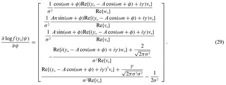
Due to the complicated integral ofvnin (20), the closed-form expression of (29) is difficult to be obtained.As a result, withMMonte Carlo trials, (28) is calculated as

wheredenotes then-th observed data inm-th trial.Apparently, (30) is only an approximation of the expectation.Therefore, a sufficiently large value ofMwill make (30) approaching (28).

5 Simulation Results

To assess the proposed algorithm, several simulations have been conducted.The mean square frequencyerror(MSFE),referredtoasE{(-ω)2},is employed as the performanceme asure.Then the noise-free signalsnis generated with the use of (10) whereA= 9.33,ω= 0.76 and φ= 0.5.In the M-H algorithm, the initial estimate is set to as [11111]T, while the number of iterations isK= 8000.Here comparison with conventional estimators, such as the ℓ1-norm estimator, MLE andM-estimator [24]are provided due to its robust and suboptimal for the Cauchy noise, while the CRLB are also included asabenchmark.It is noted that theℓ1-normminizer is solved by the least absolute deviation[36],while the initial values of MLE andM-estimator are defined using fast Fourier transform.Furthermore,the stopping criterion of these three methods are relative error smaller than 10-8.Simulations are obtained by using Matlab on Intel(R) Core(TM) i7-4790 CPU@3.60 GHz in Windows 7 operation system.While all results are based on 500 Monte Carlo runs and a data length ofN= 100.

First of all, the choice of the batch-mode window lengthLfor the proposal covariance matrix is studied.Here the density parameters of ACG noise are set to γ= 0.05 and σ2= 0.5.Figs.2 and 3 shows the MSFEvs.Land the corresponding computational time.Here the computation time is measured with stopwatch timer in the simulator.It is shown that whenL≤1000, the MSFE can be aligned with CRLB, while the computational cost of the proposed algorithm becomes higher whenLincreases.Therefore, in the following test, we chooseLas 1000.

Figure 2: MSFE vs.L

Figure 3: The computational cost vs.L

Second, the convergence rate of the unknown parameters is investigated.Meanwhile, the burnin periodPcan be determined, accordingly.In this test, the density parameters are identical to the previous test.Figs.4 and 5 indicates the estimates of all unknown parameters in different iteration numberl, which are ω,A,φ,γ and σ2.It can be seen in these figures that after the first 2000 samples,the sampled data approaches the true values of unknown parameters.Therefore, the burn-in periodPcan be chosen as 2000 in this parameter setting.

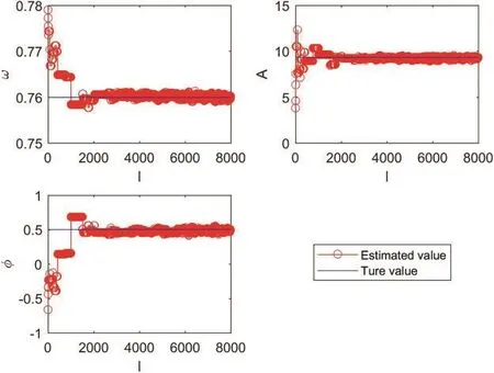
Figure 4: Estimates of unknown parameters vs. iteration number k

Figure 5: Estimates of density parameters vs. iteration number l

Finally, the MSFE of the proposed estimator is considered.In this test, all parameters are chosen as the same with the previous test.As there is no finite variance for ACG noise [18], the signal-to-noise is difficult to be defined.Therefore, here γ is scaled to produce different noise conditions.According to the study in the previous test, we throw away first 2000 samples to guarantee the stationary of the Markov chain.It is observed in Fig.6 that the MSFE of the proposed method can attain the CRLB when γ∈[-20,10] dB.Furthermore, the proposed algorithm is superior to the other three estimators,since it still can work well in higher γ.

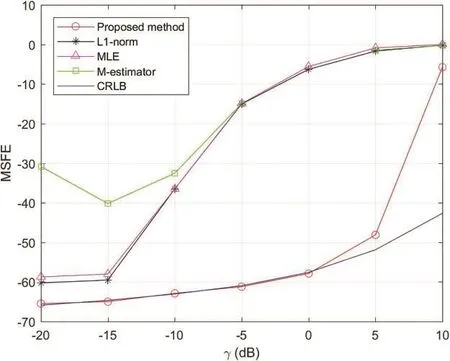
Figure 6: Mean square frequency error of ω vs.γ

6 Conclusion

In this paper, with the use of the M-H algorithm, a robust parameter estimator of a single sinusoid has been developed, in the presence of additive Cauchy-Gaussian noise.Meanwhile, a new proposal covariance updating criterion is also devised by employing the squared error of the batch-mode M-H samples.It is shown in simulation results that the developed estimator can attain the CRLB with a stationary M-H chain, indicating the accurate of our scheme.In the future work, the method can be extended to the signals with more complicated models.

Funding Statement:The workwas supported by National Natural Science Foundation of China (Grant No.52075397, 61905184, 61701021) and Fundamental Research Funds for the Central Universities(Grant No.FRF-TP-19-006A3).

Conflicts of Interest:The authors declare that they have no conflicts of interest to report regarding the present study.