Probability density functions of quantum mechanical observable uncertainties

Lin Zhang, Jinping Huang, Jiamei Wang and Shao-Ming Fei

1 Institute of Mathematics, Hangzhou Dianzi University, Hangzhou 310018, China

2 Department of Mathematics, Anhui University of Technology, Ma Anshan 243032, China

3 School of Mathematical Sciences, Capital Normal University, Beijing 100048, China

Abstract We study the uncertainties of quantum mechanical observables, quantified by the standard deviation(square root of variance)in Haar-distributed random pure states.We derive analytically the probability density functions (PDFs) of the uncertainties of arbitrary qubit observables.Based on these PDFs,the uncertainty regions of the observables are characterized by the support of the PDFs.The state-independent uncertainty relations are then transformed into the optimization problems over uncertainty regions, which opens a new vista for studying stateindependent uncertainty relations.Our results may be generalized to multiple observable cases in higher dimensional spaces.

Keywords: uncertainty of observable, probability density function, uncertainty region, statindependent uncertainty relation

1.Introduction

The uncertainty principle rules out the possibility to obtain precise measurement outcomes simultaneously when one measures two incomparable observables at the same time.Since the uncertainty relation is satisfied by the position and momentum [1], various uncertainty relations have been extensively investigated[2–7].On the occasion of celebrating the 125th anniversary of the academic journal ‘Science’, the magazine listed 125 challenging scientific problems [8].The 21st problem asks: Do deeper principles underlie quantum uncertainty and nonlocality? As uncertainty relations play significant roles in entanglement detection [9–14] and quantum nonlocality [15], and many others, it is desirable to explore the mathematical structures and physical implications of uncertainties in more detail from various perspectives.

The state-dependent Robertson–Schrödinger uncertainty relation [16–19] is of the form:

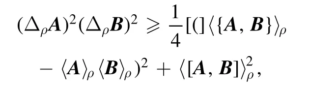
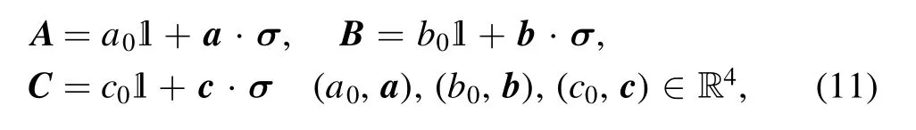
where {A,B} :=AB+BA, [A, B]:=AB −BA, and(ΔπX)2:= Tr (X2π) -Tr (Xπ)2is the variance of X with respect to the state ρ, X=A, B.

Recently, state-independent uncertainty relations have been investigated [10, 12], which have direct applications to entanglement detection.In order to get state-independent uncertainty relations, one considers the sum of the variances and solves the following optimization problems:

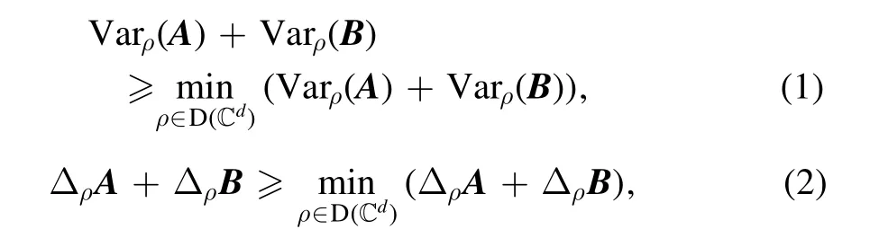
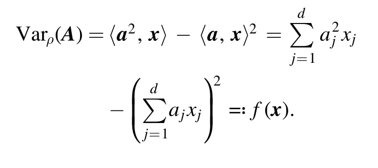
where Varπ(X) = (ΔπX)2is the variance of the observable X associated with stateπ∈ D ( Cd).

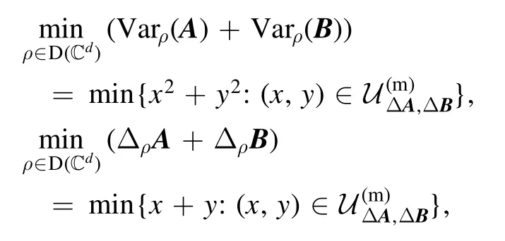
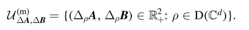
Efforts have been devoted to providing quantitative uncertainty bounds for the above inequalities [20].However,searching for such uncertainty bounds may not be the best way to get new uncertainty relations [21].Recently, Busch and Reardon-Smitha proposed to consider the uncertainty region[20]of two observables A and B,instead of finding the bounds based on some particular choice of uncertainty functional, typically such as the product or sum of uncertainties [22].Once we can identify what the structures of uncertainty regions are, we can infer specific information about the state with minimal uncertainty in some sense.In view of this,the above two optimization problems(1)and(2)become

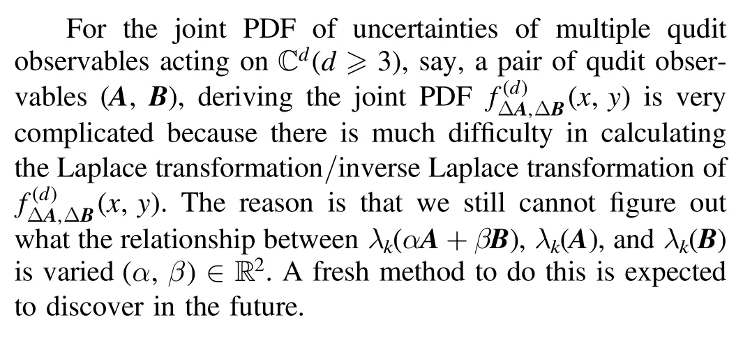
Random matrix theory or probability theory are powerful tools in quantum information theory.Recently, the nonadditivity of quantum channel capacity[23]has been cracked via probabilistic tools.The Duistermaat–Heckman measure on moment polytope has been used to derive the probability distribution density of one-body quantum marginal states of multipartite random quantum states [24, 25] and that of classical probability mixture of random quantum states[26, 27].As a function of random quantum pure states, the probability density function (PDF) of the quantum expectation value of an observable is also analytical calculated [28].Motivated by these works, we investigate the joint PDFs of uncertainties of observables.By doing so,we find that it is not necessarily to solve directly the uncertainty regions of observables.It is sufficient to identify the support of such PDF because PDF vanishes exactly beyond the uncertainty regions.Thus all the problems are reduced to compute the PDF of uncertainties of observables since all information concerning uncertainty regions and state-independent uncertainty relations are encoded in such PDFs.In [29] we have studied such PDFs for the random mixed quantum state ensembles, where all problems concerning qubit observables are completely solved,i.e.analytical formulae of the PDFs of uncertainties are obtained, and the characterization of uncertainty regions over which the optimization problems for stateindependent lower bound of the sum of variances is presented.In this paper, we will focus on the same problem for random pure quantum state ensembles.

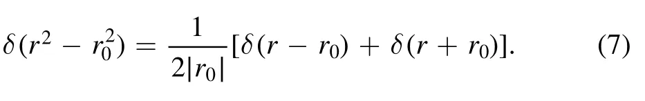
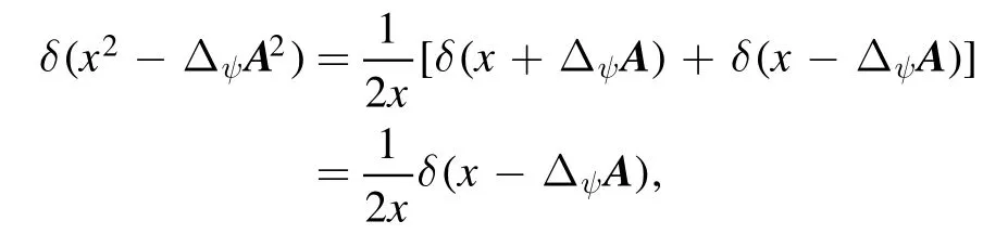
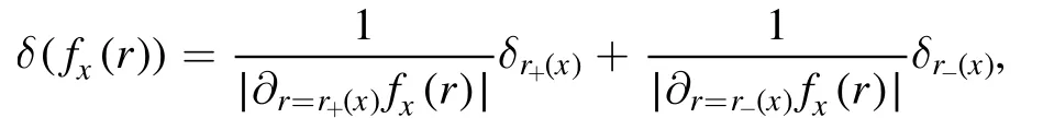
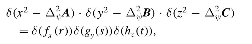
Let δ(x) be delta function [30] defined by

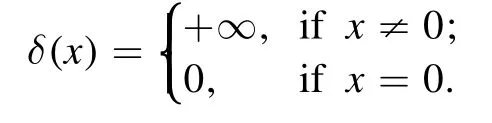
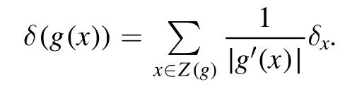
One has 〈δ,f〉:= ∫Rf(x)δ(x) dx=f(0 ).Denote by δa(x):=δ(x −a).Then 〈δa,f〉 =f(a).Let Z(g):={x ∈D(g):g(x)=0}be the zero set of function g(x)with its domain D(g).We will use the following definition.

Definition 1.[31, 32]

Ifg: R→R is a smooth function (the first derivativeg′is a continuous function) such thatZ(g) ∩Z(g′) = ∅, then the compositeδ◦gis defined by:

2.Uncertainty regions of observables

We can extend the notion of the uncertainty region of two observables A and B,put forward in[20],into that of multiple observables.

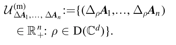
Definition 2.Let(A1,…,An)be an n-tuple of qudit observables acting ondC .The uncertainty region of such n-tuple(A1,…,A n), for the mixed quantum state ensemble, is defined by

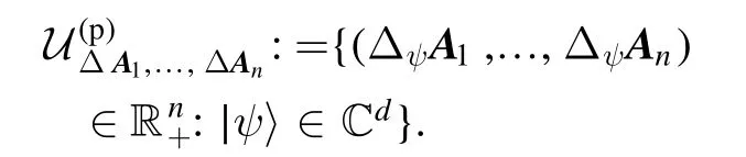
Similarly, the uncertainty region of such n-tuple(A1,…,A n),for the pure quantum state ensemble, is defined by

Note that our definition of the uncertainty region is different from the one given in [2].In the above definition, we use the standard deviation instead of variance.

Proposition 1.It holds that

is a closed interval [0, maxψVarψ(A)].

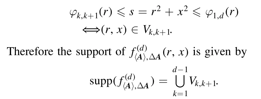
Proof.Note that P(A) ⊂ M(A) ⊂conv( P (A)).Here the first inclusion is apparently; the second inclusion follows immediately from the result obtained in [33]: for any density matrixπ∈ D ( Cd)and a qudit observableA, there is a pure state ensemble decompositionsuch that

Since all pure states onCdcan be generated via a fixedψ0and the whole unitary groupU (d), it follows that

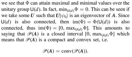
Therefore

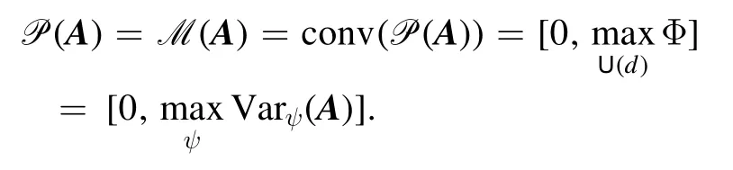
This completes the proof. □

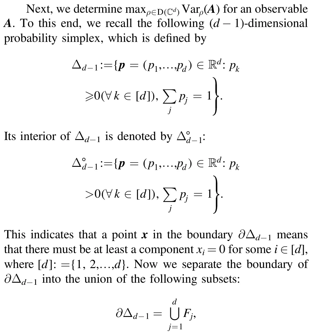
where Fj:={x ∈∂Δd−1:xj=0}.Although the following result is known in 1935 [34], we still include our proof for completeness.

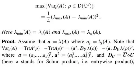
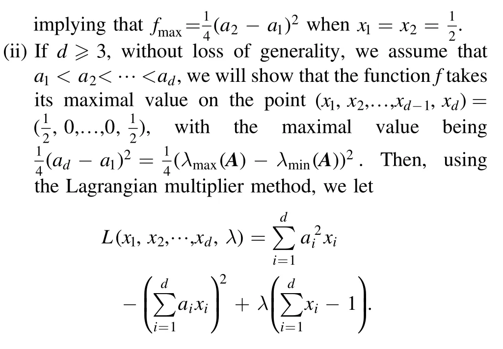
Proposition 2.Assume thatAis an observable acting ondC .Denote the vector consisting of eigenvalues ofAbyλ(A)with components beingλ1(A) ≤ …≤λd(A).It holds that

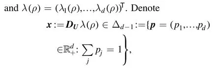
the(d-1) -dimensional probability simplex.Then

(i) If d=2,

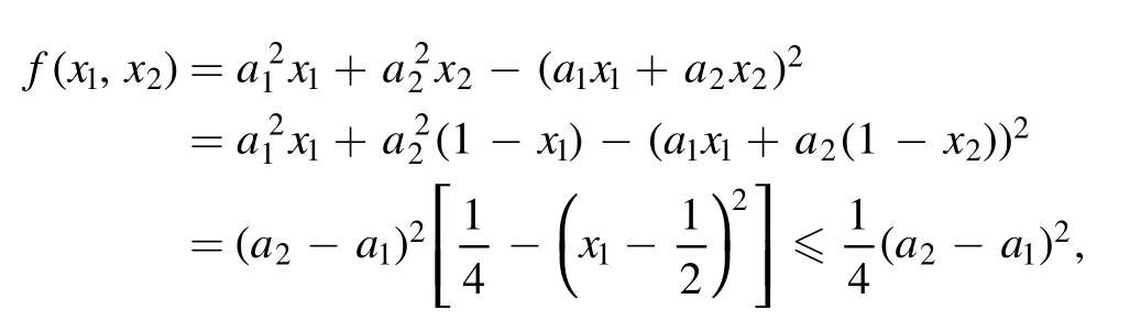
Thus

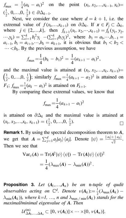
Proof.The proof is easily obtained by combining proposition 1 and proposition 2. □

3.PDFs of expectation values and uncertainties of qubit observables

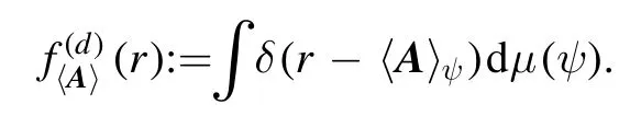
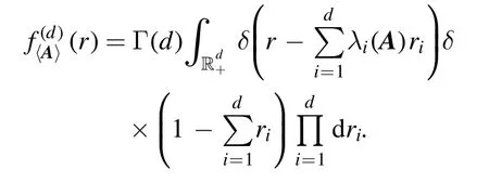
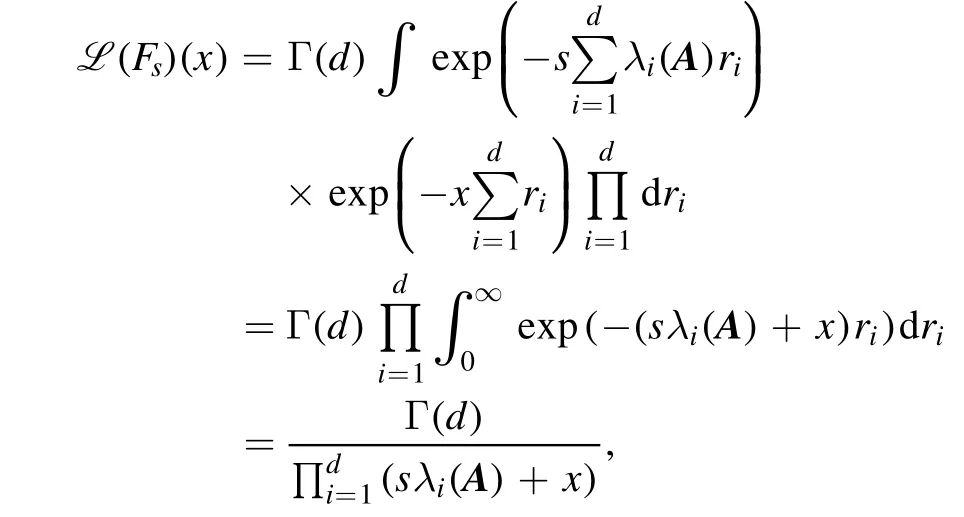
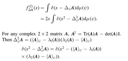
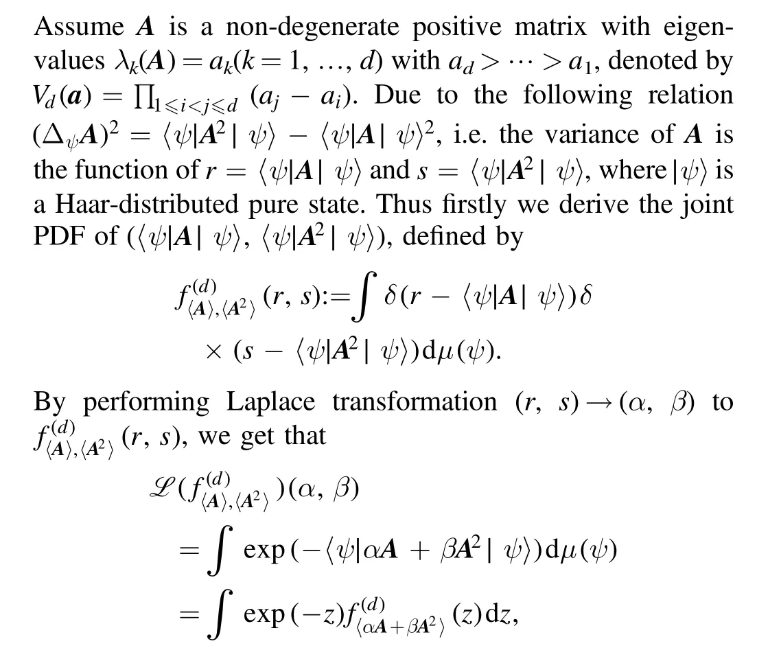
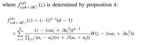
Assume A is a non-degenerate positive matrix with eigenvalues λ1(A)＜…＜λd(A), denoted by λ(A)=(λ1(A), …,λd(A)).In view of the specialty of pure state ensemble and noting propositions 1 and 2, we will consider only the variances of observable A over pure states.In fact, the same problem is also considered very recently for mixed states[29].Then the PDF of〈A〉ψ:= 〈ψ∣A∣ψ〉is defined by

Here dμ(ψ) is the so-called uniform probability measure,

which is invariant under the unitary rotations, and can be realized in the following way:

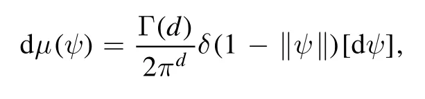
where [dψ]=for ψk=xk+iyk(k=1, …, d),and Γ(·) is the Gamma function.Thus

For completeness,we will give a different proof of it although the following result is already obtained in [28]:

Still by performing Laplace transformation(t→x)of Fs(t):

implying that [35]

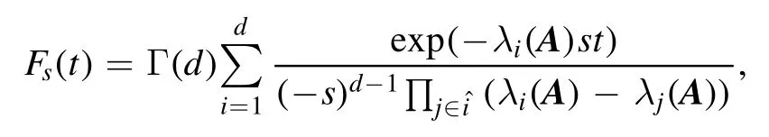
where:={ 1 ,…,d} {i}.Thus

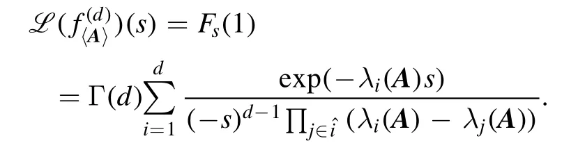
Therefore, we get that

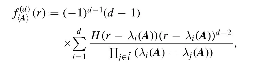
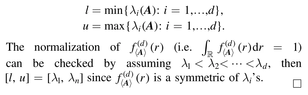
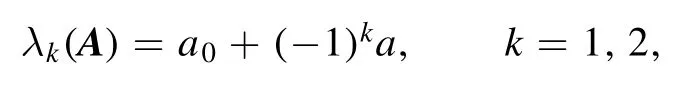
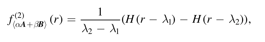
whereH(r-λi(A))is the so-called Heaviside function,defined byH(t) = 1ift＞ 0;otherwise 0.The support of this pdf is the closed interval[l,u]where

3.1.The case for one qubit observable

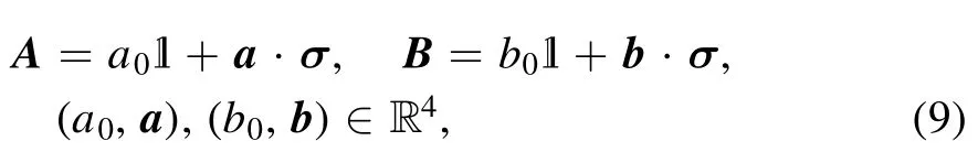
Let us now turn to the qubit observables.Any qubit observable A, which may be parameterized as

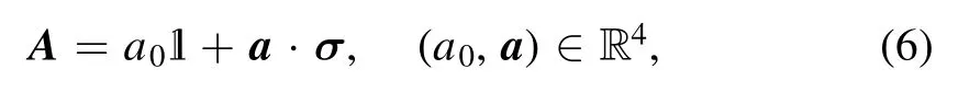
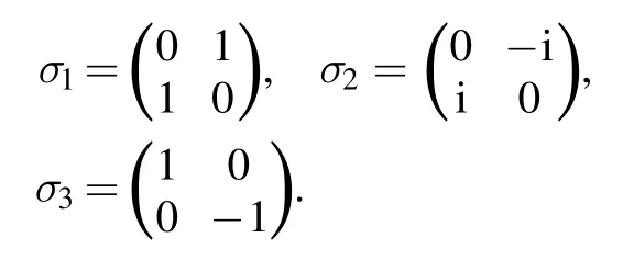
where 1 is the identity matrix on the qubit Hilbert space2C ,and σ=(σ1, σ2, σ3) is the vector of the standard Pauli matrices:

Without loss of generality, we assume that our qubit observables are of simple eigenvalues, otherwise the problem is trivial.Thus the two eigenvalues of A are

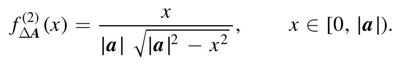
Theorem 1.For the qubit observableAdefined by equation(6),the PDF ofΔψA,where ψ is a Haar-distributed random pure state on2C , is given by

Proof.Note that

Forx≥0 , because

we see that

In particular, we see that

Thus

implying that

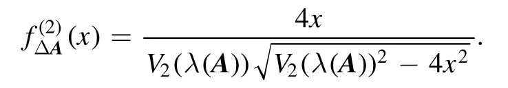
Now forA=a01+a·σ, we haveV2(λ(A) ) = 2∣a∣.Substituting this into the above expression,we get the desired result:

wherex∈[0 ,∣a∣).This is the desired result. □

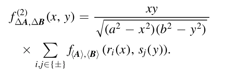
3.2.The case for two-qubit observables

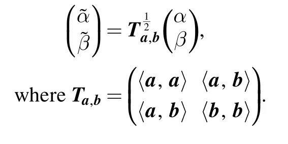
Let A=a0+a·σ and B=b0+b·σ

where

for

Now that

therefore

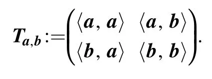
(i) If{a,b} is linearly independent, then the following matrix Ta,bis invertible, and thus

Thus we see that

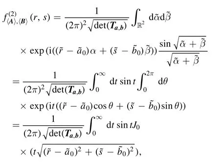
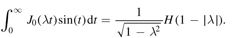
where J0(z) is the so-called Bessel function of the first kind, defined by

Therefore

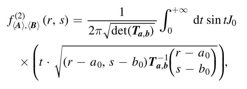
where

Therefore

where

(ii) If{a,b}is linearly dependent, without loss of generality, let b=k·a for some nonzero k ≠0, then

Herea=∣a∣ .We perform the change of variables(α,β) → (α′ ,β′) , whereα′ =α+kβandβ′ =β.We get its Jacobian, given by

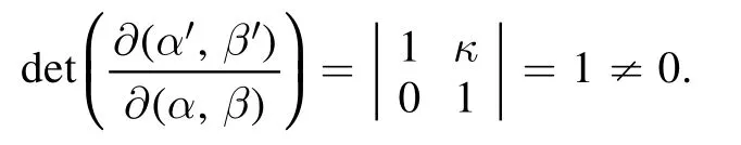
Thus

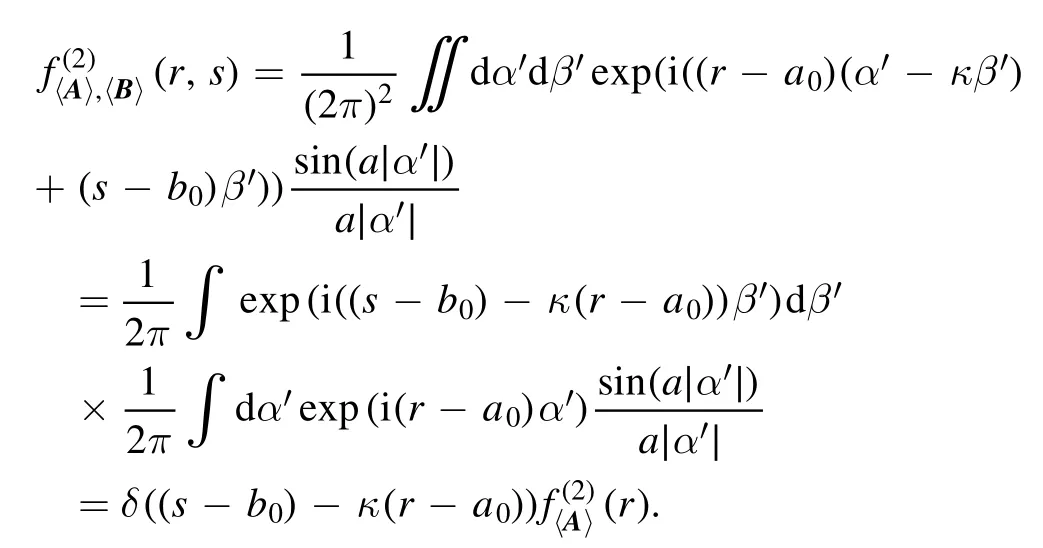
(ii) If{a,b}is linearly dependent, without loss of generality, letb=k·a, then

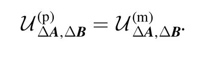
From proposition 5, we can directly infer the results obtained in [36, 37].

We now turn to a pair of qubit observables

whose uncertainty region

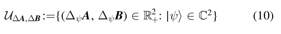
was proposed by Busch and Reardon-Smith[20]in the mixed state case.We consider the probability distribution density

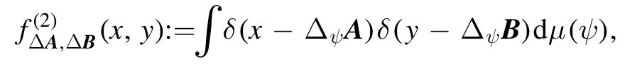
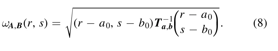
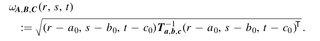
on the uncertainty region defined by equation (10).Denote

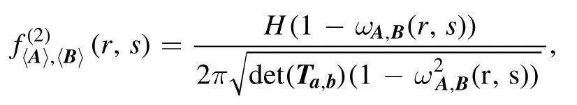
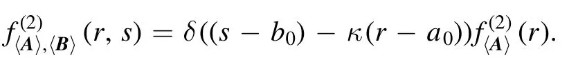
Theorem 2.The joint probability distribution density of the uncertainties (ΔψA, ΔψB)for a pair of qubit observables defined by equation (9), where ψ is a Haar-distributed random pure state on2C , is given by

Proof.Note that in the proof of theorem 1, we have already obtained that

From the above, we have already known that

Based on this observation, we get that

It is easily checked thatωA,B(·,·), defined in (8), satisfies that

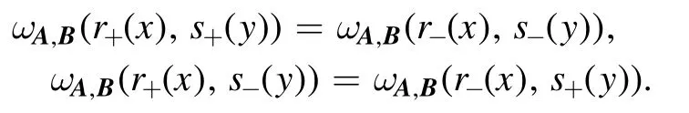
These lead to the fact that

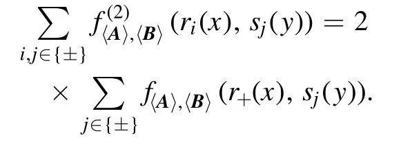
Therefore

We get the desired result. □

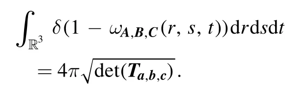
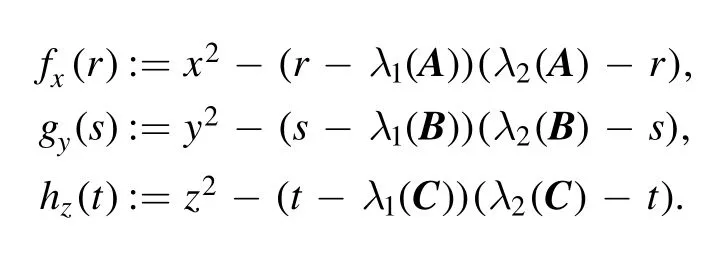
3.3.The case for three-qubit observables

We now turn to the case where there are three-qubit observables

whose uncertainty region

We define the probability distribution density

on the uncertainty region defined by equation (12).Denote

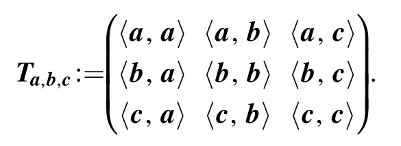
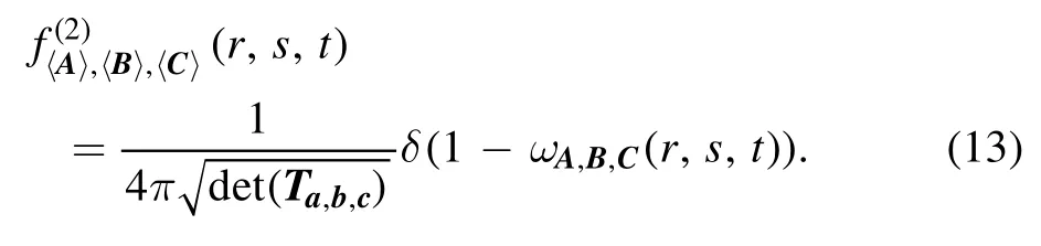
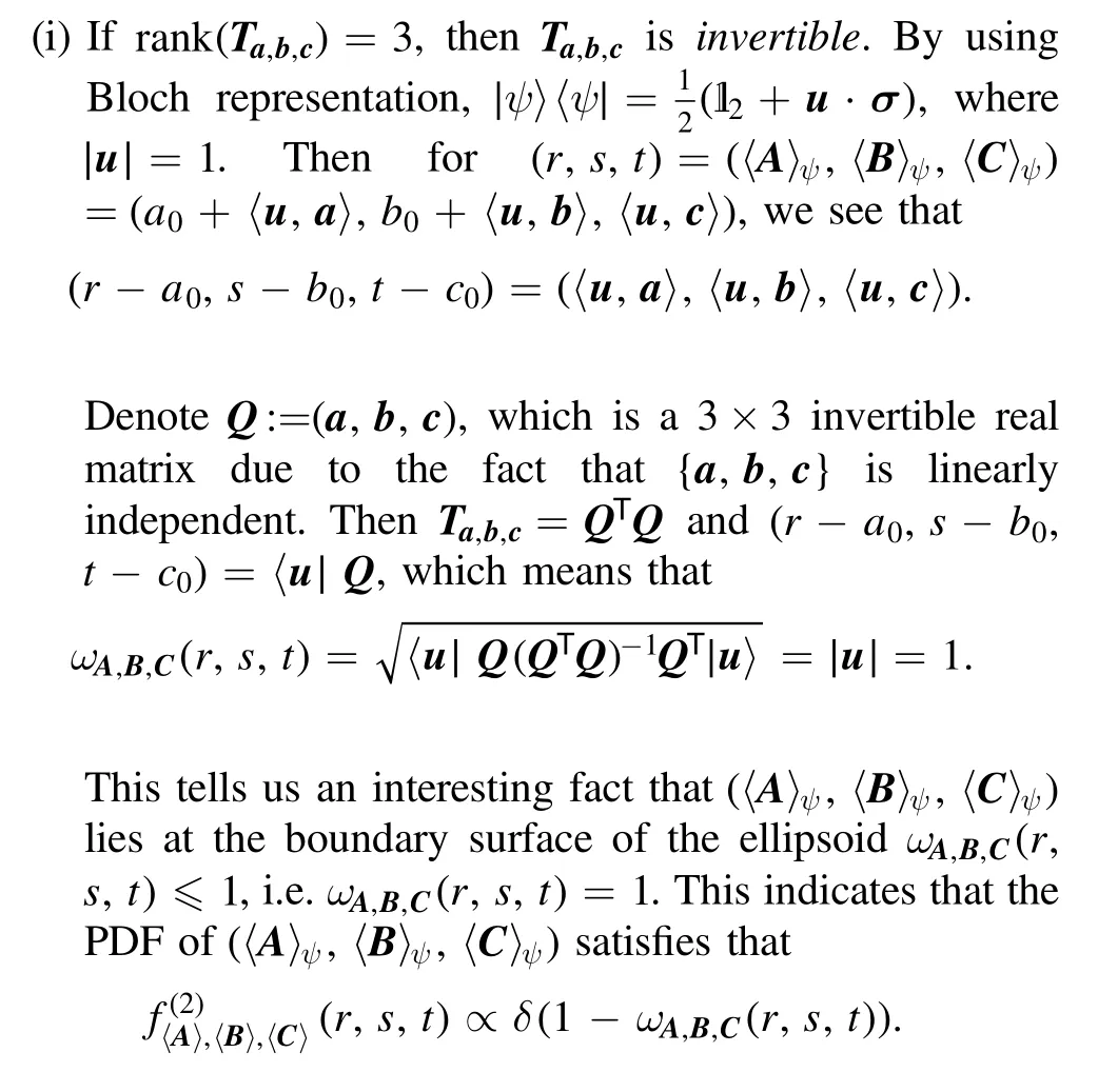
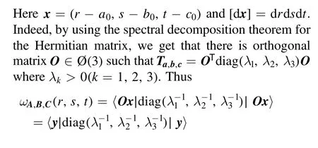
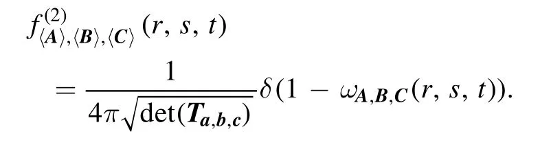
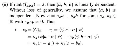
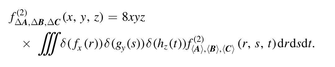
Again note that Ta,b,cis also a semidefinite positive matrix.We find that rank(Ta,b,c)≤3.There are three cases that would be possible:rank(Ta,b,c)=1,2,3.Thus Ta,b,cis invertible(i.e.rank(Ta,b,c)=3) if and only if{a,b,c}linearly independent.In such case, we write

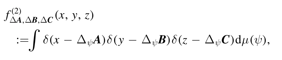
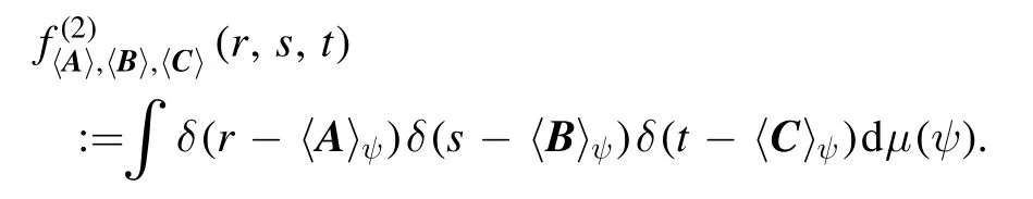
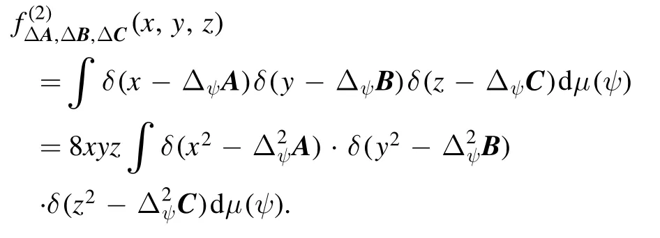
In order to calculate fΔA,ΔB,ΔC, essentially we need to derive the joint probability distribution density of (〈A〉ψ, 〈B〉ψ,〈C〉ψ), which is defined by

We have the following result:

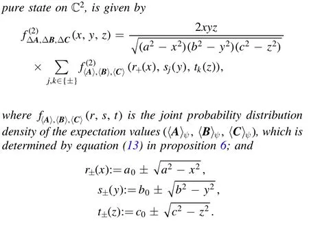
Proposition 6.For three-qubit observables, given by equation (11), (i) ifrank(Ta,b,c) = 3, i.e.{a,b,c} is linearly independent, then the joint probability distribution density of(〈A〉ψ, 〈B〉ψ,〈C〉ψ), where ψ is a Haar-distributed random pure state on2C , is given by the following:

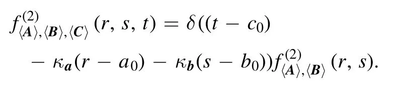
(ii) Ifrank(Ta,b,c) = 2, i.e.{a,b,c} is linearly dependent,without loss of generality, we assume that{a,b} is linearly independent andc=ka·a+kb·bfor somekaandkbwithk a kb≠ 0, then

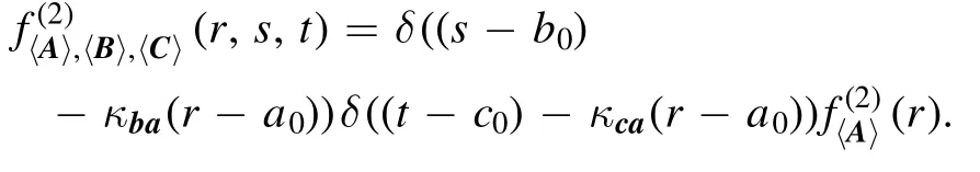
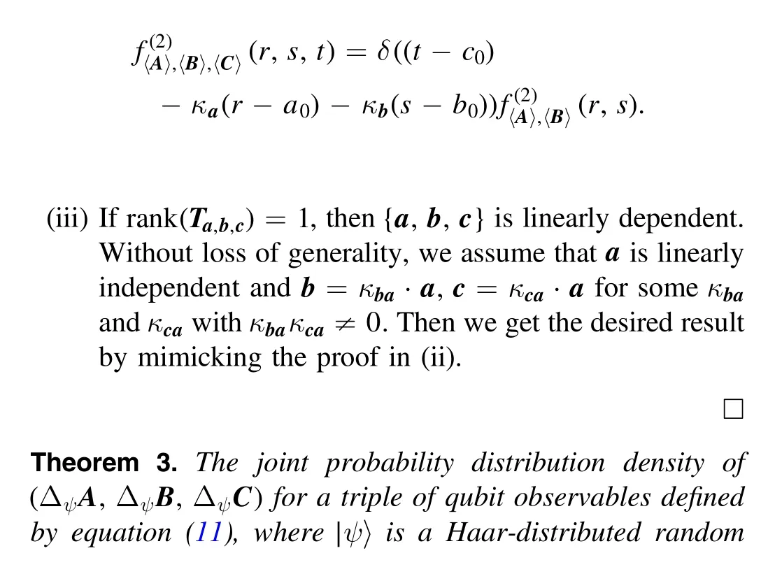
(iii) Ifrank(Ta,b,c) = 1, i.e.{a,b,c} is linearly dependent,without loss of generality,we assume thataare linearly independent andb=kba·a,c=kca·afor somekbaandkcawithk ba kca≠ 0, then

Proof.

Next, we calculate the following integral:

Apparently

wherey=Ox.Thus

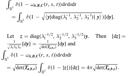
Finally, we get that

Therefore we get that

Proof.Note that

Again using the method in the proof of theorem 1, we have already obtained that

where

Then

Furthermore, we have

Based on this observation, we get that

Thus

It is easily seen that

From these observations,we can reduce the above expression to the following:

The desired result is obtained. □

Note that the PDFs of uncertainties of multiple qubit observables (more than three) will be reduced into the three situations above,as shown in[29].Here we will omit it here.

4.PDF of uncertainty of a single qudit observable

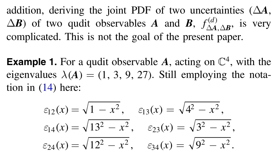
Theoretically, we can calculate the above integral for any finite natural number d,but instead,we will focus on the case where d=3, 4, we use Mathematica to do this tedious job.By simplifying the results obtained via the Laplace transformation/inverse Laplace transformation in Mathematica, we get the following results without details.

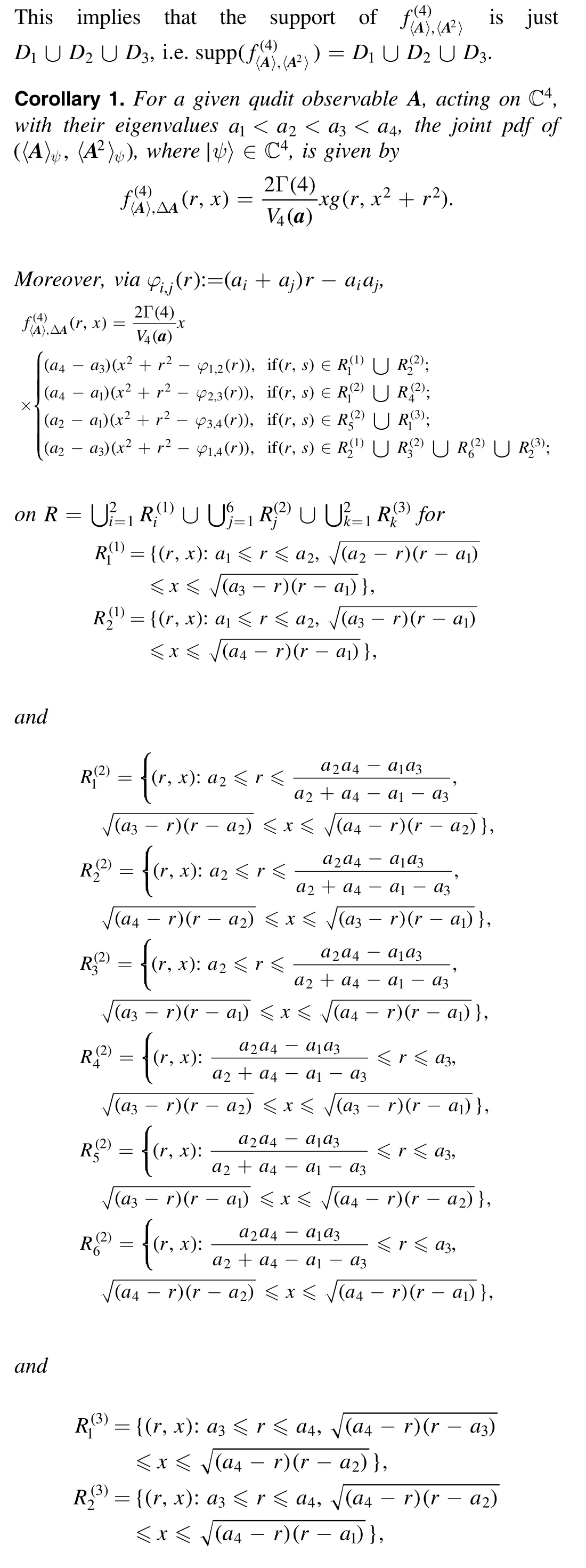
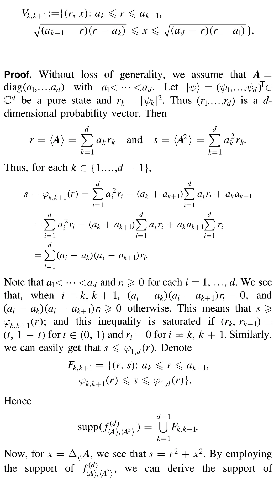
Figure 1.Plots of the supports of for qudit observables A.

Here the meanings of the notations χ andεijcan be found in theorem 4.

Then from corollary 1,using marginal integral,we can derive the PDF ofΔψAthat

(i) Ifx∈[0, 1], then

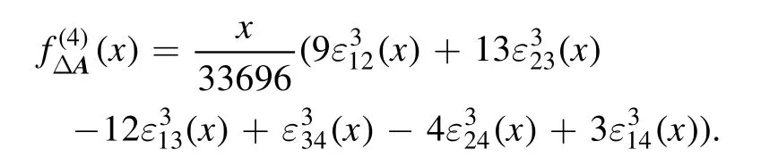
(ii) Ifx∈[1, 3], then

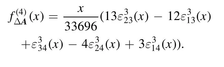
(iii) Ifx∈[3, 4], then

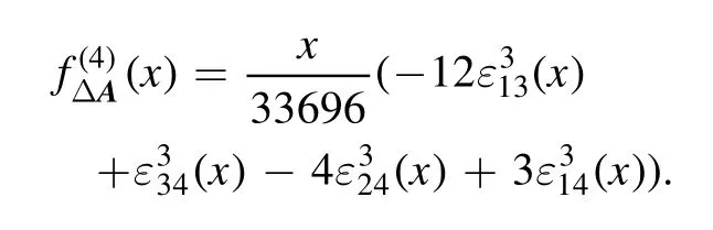
(iv) Ifx∈[4, 9], then

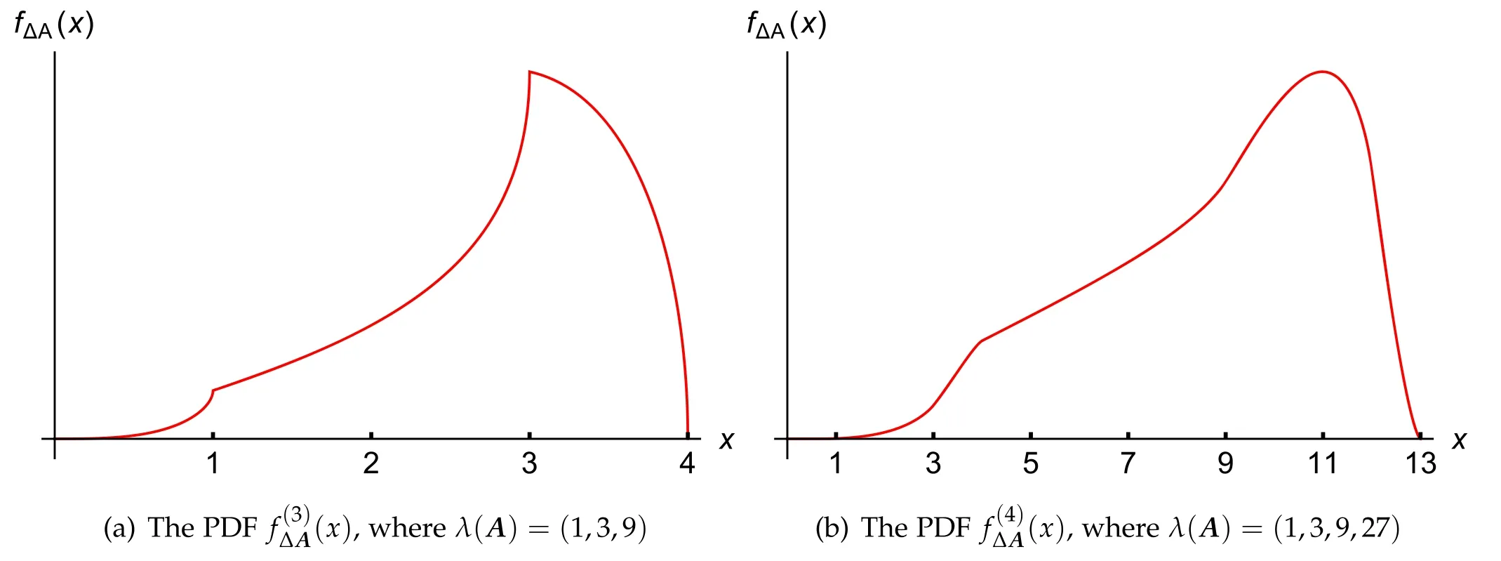
Figure 2.Plots of the PDFs for qudit observables A.

where

then

This completes the proof.

5.Discussion and concluding remarks

which is exactly the one we obtained in[29]for mixed states.This indicates that, in the qubit situation, we have that

Proposition 7.For a pair of qubit observables(A,B) acting on C2, it holds that

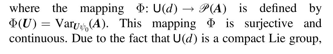
One may wonder if this identity holds for general d ≥2,as the variance of A with respect to a mixed state can always be decomposed as a convex combination of some variances of A associated with pure states, see equation (3).

We hope the results obtained in the present paper can shed new light on the related problems in quantum information theory.Our approach may be applied to the study of PDFs in higher dimensional spaces.It would also be interesting to apply PDFs to measurement and/or quantum channel uncertainty relations.

Acknowledgments

This work is supported by the NSF of China under Grant Nos.11 971 140, 12 075 159, and 12 171 044, Beijing Natural Science Foundation (Z190005), the Academician Innovation Platform of Hainan Province, and Academy for Multidisciplinary Studies, Capital Normal University.LZ is also funded by Natural Science Foundations of Hubei Province Grant No.2020CFB538.