Extreme Wind Variability and Wind Map Development in Western Java, Indonesia
2022-08-02MuhammadRaisAbdillahPrasantiWidyasihSarliHafidzRizkyFirmansyahAnjarDimaraSaktiFaizRohmanFajaryRobiMuharsyah
Muhammad Rais Abdillah · Prasanti Widyasih Sarli · Hafidz Rizky Firmansyah ·Anjar Dimara Sakti · Faiz Rohman Fajary · Robi Muharsyah ·
Gian Gardian Sudarman8,9
Abstract Wind-related disasters are one of the most frequent disasters in Indonesia.It can cause severe damages of residential construction, especially in the world’s most populated island of Java. Understanding the characteristics of extreme winds is crucial for mitigating the disasters and for defining structural design standards. This study investigated the spatiotemporal variations of extreme winds and pioneered a design wind map in Indonesia by focusing on western Java. Based on gust data observed in recent years from 24 stations, the extreme winds exhibit a clear annual cycle where northwestern and southeastern sides of western Java show out-of-phase relationship due to reversal monsoons. Meanwhile, extreme wind occurrences are mostly affected by small-scale weather systems, regardless of seasons and locations. To build the wind map, we used bias-corrected gust from ERA5 and applied the Gumbel method to predict extreme winds with different return periods. The wind map highlights some drawbacks of the current national design standards, which use single wind speed values regardless of location and return period.Beside a fundamental improvement for wind design, this study will benefit disaster risk mapping and other applications that require extreme wind speed distribution.
Keywords ERA5 reanalysis · Extreme wind · Mixed weather system · Tropical climate
1 Introduction
The Indonesian National Disaster Management Authority1BNPB (Badan Nasional Penanggulangan Bencana) is the Indonesian name of the National Disaster Management Authority.reported that strong wind events have been a major contributor to disasters in Indonesia (BNPB 2021). In the past decade, strong wind has consistently been the second or third source of hazard, prompting the needs to understand the nature of wind in the region.Not only structures,power and communication networks are particularly vulnerable,with many slender structures being wind sensitive, whose failure can have a significant socioeconomic impact. Furthermore, there is an increasing number of tall buildings and long span bridges in the region for which wind loading is particularly important.
The current Indonesian design standards do not have a consistent value for wind loading,and they typically assign a singular value to the whole region. In the earlier design standard for buildings, the Ministry of Public Works(PPPURG)2PPPURG (Pedoman Perencanaan Pembebanan untuk Rumah dan Gedung) is the old loading standard for general buildings. It was published by the Ministry of Public Works or PU(Pekerjaan Umum).(PU 1987) introduced a general design wind speed of 20 m s-1for the whole region and a special speed of 25 m s-1for coastal area.This design standard is applied uniformly in the whole country and does not have a specific return period. Even more recent design standard for buildings (SNI 1727-2020)3SNI (Standar Nasional Indonesia) is the Indonesian National Standardization, which is published under BSN (Badan Standarisasi Nasional).(BSN 2020) does not specify any design wind speed. In the design standard for bridges(SNI 1725-2016)(BSN 2016),the design wind speed is set between 25 to 35 m s-1for low to high wind speed regions,although these regions are not specified within the map.
The Australian standard of HB212-2002 Design Wind Speeds for the Asia-Pacific Region (Holmes and Weller 2002) assigns the whole Indonesia to a design wind speed of Level 1.According to this standard,the 50-year and the 500-year return periods wind speeds are 32 and 40 m s-1,respectively. However, the design wind speeds have several problems:(1)they are used in the equatorial region as a single value; (2) only a few stations (11 stations) was involved in the study for the whole equatorial region; (3)the exact location of the stations is unclear, preventing an assessment of regional representativeness;and(4)the study result may be outdated as it was done 20 years ago.
Due to a lack of a regionally-dependent design wind map, in practice local engineers gather wind data from the Indonesian Meteorological, Climatological, and Geophysical Agency (BMKG)4BMKG (Badan Meteorologi Klimatologi dan Geofisika) is responsible for operational weather observations in Indonesia.on their own (BSN 2020). The engineers typically collect wind data from a conventional meteorological station closest to their desired location.Unfortunately conventional meteorological stations in Indonesia are relatively scarce. The engineers often question the representativeness of the observed wind data utilized for their designs. Moreover, the official data only provide hourly mean wind speed, whose value is fundamentally much lower than gust speed. The available observation period is also limited, ranging from several years to more than a decade, while the design wind speed needed by civil engineers typically has a much longer return period (Pintar et al. 2015). These limitations contribute to inaccurate design wind speed values.
Another concern comes from the minimum research available in understanding extreme wind in the region.Many studies were done in regions where tropical cyclones(TC)pass regularly,such as in Vietnam,Philippines,Japan,and China (Garciano et al. 2005; Pacheco et al. 2005;Ishihara and Yamaguchi 2015; Zheng et al. 2020; Nguyen et al. 2021), but only few studies have been performed in non-TC regions of Southeast Asia. Choi and Tanurdjaja(2002) showed that in the case of Singapore, which has a mixed weather system, the extreme wind speed is generated by both large-scale and small-scale meteorological drivers. However, the mechanisms of extreme wind in Indonesia might differ and vary accross the region.Understanding these characteristics becomes indispensable to have a proper design wind speed analysis in Indonesia.
This study aimed to investigate the variability of extreme wind and develop a new regionally-dependent wind map for structural design by focusing on the western side of Java Island. This region is very vulnerable to wind disaster because it has the highest population density.This article is organized as follows. Section 2 presents data and methods used in this study. Section 3 shows the results.Section 4 discusses the benefit and limitation of the current study. Section 5 summarizes the important findings and future implications.
2 Data and Methodology
This section is divided into Data and Method. The former shows basic datasets including meteorological station and reanalysis data.The latter consists of four general steps that allow us to examine variabilities of extreme wind speed and to build a wind map.
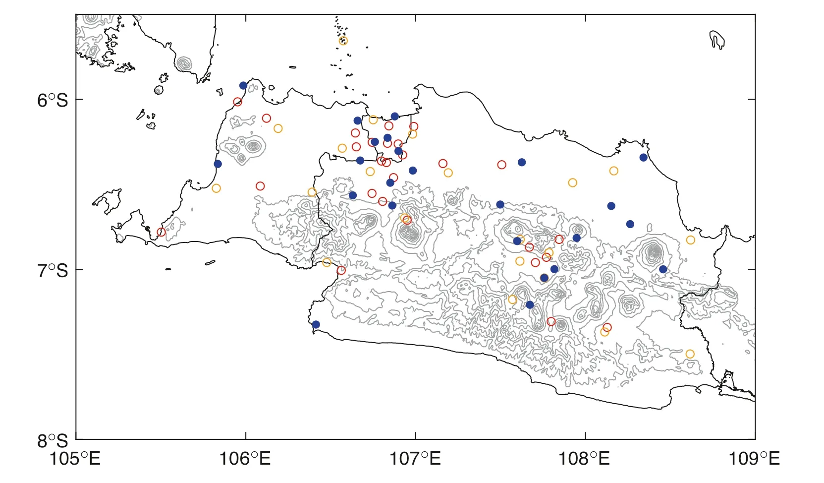
Fig. 1 Map of western Java superimposed with wind measurement stations (circles)and topography with a contour interval of 250 m (thin black contour).Blue circles denote the stations that passed all quality control (QC) steps. Red and orange circles denote the stations that did not pass the first and the second steps of QC,respectively. Thick black lines denote coastlines and administrative boundaries
2.1 Data
The meteorological datasets are obtained from local automatic weather stations (AWS) and a climate reanalysis.This section briefly describes the availibility, quality, resolution, and other specifications of these data.
2.1.1 Station Data
The wind data are collected from 64 AWS operated by BMKG over five years (2016—2020) covering three provinces in western Java: Banten, DKI Jakarta, and West Java. The recorded AWS data offer 10-min mean wind speed and maximum wind speed (that is, gust speed) at 10 m height. To add more wind observations, we incorporate data from eight additional AWS deployed by Institut Teknologi Bandung and Durham University. A total of 72 stations are used (Fig. 1).
2.1.2 Reanalysis Data
The collected observation data cover only five years. To analyze extreme values in a longer period, we use wind data from an atmospheric reanalysis.Reanalyses provide a 3D global atmospheric dataset constructed from assimilating numerous observations into the state-of-the-art global climate models.Vajda et al.(2011)evaluated gust data from ERA-interim reanalysis(Dee et al.2011)and found a good agreement between daily observed maximum gust and reanalysis gust. Zheng et al. (2020) used the ERAinterim gust to calculate extreme wind speed with return periods of 50-year and 100-year in the China seas.
Recently, the European Centre for Medium-Range Weather Forecasts (ECMWF) released their latest reanalysis called ERA5(Hersbach et al.2020).ERA5 is available every 1 hour at 0.25°horizontal resolution.The resolutions are generally better compared with other reanalyses. Minola et al. (2020) found that wind gust from ERA5 is generally accurate and better than its predecessor (ERAinterim) although there are some discrepancies with observation over complex topography.In this study,we use the hourly gust of ERA5 from 1979 to 2020 (42 years).ERA5 gust is parameterized from surface stress, surface friction,wind shear,and atmospheric stability.We also use monthly average of wind speed data at 925 hPa to show prevailing wind in each season.
2.2 Method
First,a series of quality control(QC)procedures is applied to filter out any suspected records in station data.Data that pass the QC are then used to analyze spatiotemporal variabilities of extreme wind speed and gust observations.After that we calibrate ERA5 gust and develop a design wind map.
2.2.1 Quality Control of Station Data
The quality of observed wind data is evaluated by two major steps of QC.The first step consists of two checks:(1)checking the availability of wind data and(2)checking the quality of wind distribution. Our study focuses on daily maximum wind calculated from 10-min maximum wind speed (also referred to as daily gust and maximum gust in text). We also calculate daily mean wind speed for adynamic evaluation in the second QC step. The daily statistics are calculated only for days having at least 70%of data in a day or 70% of data in the afternoon (12—21 local time). The afternoon time window is set because most of daily maxima appear during this period due to diurnal cycle influence. Darman (2019) reported that most of the windinduced disasters in Indonesia occurred in the afternoon.We exclude stations having less than 365 days of daily wind data. To check the quality of wind distribution, an empirical cumulative distribution function (CDF) graph is inspected and a station is flagged if:(1)the median of data is either too low or too high compared with other stations or (2) there are many data concentrated in the end tails of CDF (for example, a sharp increase of CDF in the lowest 5th percentile or highest 95th percentile that appears likely due to repetitions). The flagged stations are suspected to suffer from incomplete calibration or instrument errors and thus excluded from the analysis.From a total of 72 stations,45 stations pass the first step of QC and are transferred to the second step of QC.

Table 1 List of stations that passed the QCs and statistics of the observed daily average wind speed and daily maximum gust speed
The second step of QC is done to assess dynamic criteria of wind maximum. This step follows a QC procedure of wind gust documented by Cha´vez-Arroyo and Probst(2015). The QC consists of three main checks: plausible value check, internal consistency check, and temporal consistency check. The plausible value check ensures that the observed wind data are within the instrument limit and dynamic limit. The instrument limit depends on each manufacturer, while the dynamic limit states that the daily gust must be well fitted by a Generalized Extreme Value(GEV) distribution. The internal consistency check deals with the relation between wind speed and gust such that the daily maximum must be higher than the daily average wind speed.The temporal consistency check aims to find data of abnormally high variations indicated by the relationship between daily mean wind and daily gust. This check is important to objectively separate extreme values and suspected outliers. Details of the method are shown in Cha´-vez-Arroyo and Probst (2015). The final check returns 24 stations that satisfy the whole QC procedure (Table 1).
2.2.2 Observational Analysis from the Station Data
We calculate the statistics of wind data at each station.The averages and 99th percentiles are computed to describe the average condition and extreme values of wind observation,respectively. Note that the definition of extreme value in this section is different from the extreme value defined in the context of design wind speed, which uses annual maxima (see Sect. 2.2.4).
As Java Island exhibits a clear annual cycle of wind and precipitation due to monsoon reversal(Aldrian and Susanto 2003; Chang et al. 2005), we classify the wind data into four seasons: December—January—February (hereafter DJF), March—April—May (MAM), June—July—August(JJA), and September—October—November (SON). Spatial variations among stations are analyzed by using scatterplot maps. Based on distribution of seasonality, we define two clusters that group the stations according to the phase of annual cycle: Cluster Northwest (NW) monsoon and Cluster Southeast (SE) monsoon. The former indicates the stations that show peaks of seasonal gust in DJF.The latter is for the stations that exhibit peaks in JJA or SON. Wind gust distributions in each category are then investigated through boxplot diagrams. The concept of extreme wind speed in different seasons was first emphasized by Zheng et al. (2020).
To examine the driving factors of strong wind events,we separate the daily maximum wind (or daily gust) into large-scale and small-scale weather events. The classifications are achieved by quantifying the individual influences of these events each day at each station. Choi and Tanurdjaja (2002) provided a general guidance to identify these events. Large-scale events are characterized by steady wind extending for several hours to days. The wind also exhibits a diurnal pattern during such events. In contrast, the small-scale wind events are recognized by a sudden sharp change in wind speed for only that particular time of occurrence.
Based on the above information, we perform a simple decomposition. Let us define a wind speed record at a particular time as
u ≡uL+uS(1)
where uLand uSare wind speed components driven by large-scale and small-scale events, respectively. uLis calculated by filtering the wind data series (u) with a 12-hour moving average. uSis then simply obtained by subtracting u with uL. We determine a small-scale (large-scale) wind event when uSvalue is higher(lower)than uL,respectively.
2.2.3 Wind Data Calibration
Prior to conducting extreme wind analyses, we have assessed the systematic errors of ERA5 daily maximum gust during the period of station data (2016—2020). Daily biases of ERA5 at each station are calculated to represent the error. The results show distinct characteristics on the error distributions of ERA5 among stations,suggesting that we could not perform a simple bias correction or calibration technique.
We use a quantile mapping method (QM) (Themeßl et al.2011) for correcting the bias of ERA5 because it can fit the distributions of simulation and observation data.The Weibull distribution is used as the basis of QM because it is superior in correcting climatic wind data (Li et al. 2019).The Weibull distribution-based QM assumes that the probability distributions of both observed and simulated wind speeds u can be approximated using a Weibull distribution (Haas et al. 2014):

We are interested in performing calibration in the whole domain of western Java.However,error quantifications are limited to the station locations, which do not cover the whole grid boxes in ERA5. To enable calibration in the whole domain, calibration parameters cobs, ccont, kobs, and kcontare spatially interpolated.A 5×5 km interpolation is used to accommodate areas with dense stations.
2.2.4 Design Wind Speed Calculation

Fig. 2 Features of annual and seasonal patterns of wind speed (left panels) and gust (right panels) (m s-1). From top to bottom: a and b annual average;c—j seasonal anomalies on c,d December—January—February (DJF), e, f March—April—May (MAM), g, h June—July—August (JJA), and i, j September—October—November (SON). The anomalies are constructed from differences with the annual average of the corresponding station. Red arrows on left panels show the mean prevailing wind (PW) of the domain on each season, calculated from the 925-hPa wind field of ERA5 reanalysis
For design applications, extreme wind speed analysis can be performed through various techniques, including:asymptotic distribution method (Fisher and Tippett 1928;Jenkinson 1955;Gumbel 1958),parent distribution method(Gomes and Vickery 1977, 1978), peak over threshold method (Weiss 1971), method of independent storms(Cook 1982), and penultimate distribution method (Cook and Harris 2004). In this study, extreme wind speed is calculated by applying the asymptotic distribution method of Gumbel to annual maxima of calibrated ERA5 over 42 years.The Gumbel method is used as in the context of this study, no previous design wind speed map was available for the region, so that the most conservative of method is desired.The general model of Gumbel distribution follows this common relationship

where xTis the extreme wind for a given return period of T,while μ and σ are the location and the scale parameters.
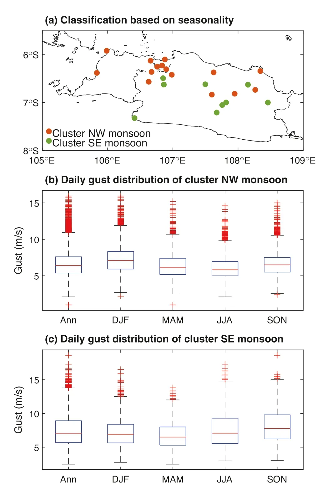
Fig. 3 Distributions of daily gust. a Classification of stations according to their annual peaks of gust. Brown and green circles are stations categorized into Cluster Northwest (NW) and Cluster Southeast (SE). b, c show annual (Ann) and seasonal distributions of daily maximum gust as boxplots. On each box, the central red line denotes the median. The bottom and top edges of the box denote the 25th (q1) and 75th (q3) percentiles, respectively. The vertical lines extend to the most extreme data points that are not classified as outliers (plotted individually using the + symbol if they are greater than q3+1.5(q3-q1) or less than q1-1.5(q3-q1)). DJF =December-January-February, MAM = March-April-May, JJA =June-July-August, SON = September-October-November
μ and σ can be calculated by using three different methods: graphical method, method of moment (MOM)(Lowery and Nash 1970), and method of L-moment(LMOM) (Vogel and Fennessey 1993). To find the best method to estimate μ and σ, root mean square error(RMSE) for all three methods are compared (El-Shanshoury and Ramadan 2012):


3 Results
The first two parts of this section present the results of station data analyses that show spatiotemporal variations of extreme wind observed in recent years and the attributions to different scales of weather events.The last part presents the new design wind map and compares it with the current standards in Indonesia.
3.1 Spatial Distribution and Seasonal Variation of Observed Wind
Statistics of the observed wind are shown in Table 1.Annual averages of wind speed range from 0.98 to 3.44 m s-1, with the whole-domain average of 1.82 m s-1. Averages of daily maximum gust are 5.32—9.95 m s-1(domain average of 6.99 m s-1). The lowest and highest 99th percentiles of daily gust are 8.58 m s-1and 15.54 m s-1,respectively. The average of the extremes is 11.64 m s-1.
The observed extreme values are generally similar to the wind speeds observed during strong wind/gust incidents in Indonesia documented in previous studies. Muzayanah(2015) reported two wind incidents with wind speed of 25—30 knots (12.86—15.4 m s-1) in East Java. Based on pilot reports in 38 airports, including those located in western Java, Rais et al. (2020) showed that near-surface gust-induced tailwind ranged from few knots up to 33 knots with a high probability at 10—20 knots(5.14—10.28 m s-1).Outside Java Island,Rinaldi(2013)and Mujiasih andPrimadi (2016) documented strong wind incidents greater than 25 knots in Borneo and Bali Islands, respectively.

Fig. 4 Attributing extreme gust occurrences (daily gust exceeding 95th percentile at each station)to the influences of small-scale (us) and large-scale(uL) weather systems. a Distribution of uL and uS for extreme gust events in all stations. b Relative roles of uL and uS on the total gust speed(u), which are denoted by the colored circles. c Probability distribution functions (pdfs) of differences between uS and uL(Δ).The pdfs are also calculated for stations grouped into Cluster NW and SE monsoons as well as December-January-February(DJF) and June-July-August(JJA) seasons. d Distribution of extreme gust events categorized into large-scale and small-scale weather-driven groups according to differences in(c) for all regions and seasons
The spatial patterns of annual wind speed and gust are quite consistent (Fig. 2a, b). Lower wind speed and gust tend to be observed in the center of the island where the mountain ranges reside(Fig.1).Higher wind speed is more dominant in the lowland and coastal areas. Note that wind speeds at some stations show large differences with their surrounding stations, possibly owing to local effects that effectively modulate the wind variation. A future study is needed to clarify this phenomenon.
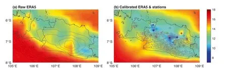
Fig. 5 Spatial comparison of a raw and b calibrated ERA5 gusts (m s-1) shown by the 99th percentiles. Brown contours in a, b show topography in ERA5 and topography in 1-km Shuttle Radar Topography Mission (SRTM) data (Sandwell et al. 2014), respectively. Circles in (b) denote gusts from stations
Seasonal anomalies in Fig. 2c—j indicate a strong and organized annual cycle of wind among the four seasons.In DJF when the prevailing wind is northwesterly, the northwestern side of the study area experiences higher wind speed and gust compared to their annual averages,whereas the southeastern side stations report lower wind speed (Fig. 2c, d). In JJA and SON, an opposite effect appears due to the prevailing southeasterly wind that results in positive and negative anomalies in the southeastern and northwestern sides, respectively (Fig. 2g—j).Meanwhile,wind anomalies in MAM tend to be negative in all stations (Fig. 2e, f), possibly due to much weaker prevailing wind in this season.
The previous analysis only discusses the variation of average values. To examine the variation of extreme values,we plot distributions of daily gust in Fig.3 and classify them into the two clusters of stations according to their seasonality. The appearance of upper outliers in boxplots indicates that the seasonality of extreme gusts is similar to the averages. For example, in the northwest region,extreme winds in DJF are generally stronger than those in JJA. This pattern is consistent with a separate study by Poerbandono(2016)who reported that extreme wind speed in the Seribu Islands (north of Jakarta) was larger during the west monsoon (DJF). In contrast, in the southeast region, the extreme winds are stronger in JJA/SON and weaker in DJF (Fig. 3). The upwind stations tend to have stronger extreme wind than the downwind stations.
3.2 Attribution to the Large-Scale and Small-Scale Weather Events
Gomes and Vickery (1978) pointed out the importance of separating extreme wind analyses in a mixed climate region. Choi (1999) followed this approach and separated the extreme events according to the associated weather systems in Singapore.The mixture of the different weather systems suggest a more complicated estimation of design wind speed because they likely have different extreme value distributions. Previous studies tend to divide the wind-producing weather systems into thunderstorm and non-thunderstorm (Choi 2000; Lombardo et al. 2009).Many strong wind incidents in Indonesia have been linked to thunderstorms (Muzayanah 2015; Nugraha and Trilaksono 2018; Rais et al. 2020). However, sorting the thunderstorm events require detailed weather reports,which are unavailable in the current stations. Choi and Tanurdjaja(2002) suggested a more appropriate approach by sorting wind data into small-scale and large-scale weather events instead of thunderstorm and non-thunderstorm events. The small-scale weather systems, such as convective instabilities, thunderstorms, and mechanical turbulence, trigger locally-relevant winds. The large-scale weather systems,for example those associated with synoptic weather patterns and monsoons,have impacts on the background wind flow.
Figure 4 shows the relative contributions of large-scale and small-scale weather events on extreme gust occurrences(gusts greater than 95th percentile at each station).It is evident that the small-scale weather events induce stronger wind compared with the large-scale events(Fig. 4a, b). The average of small-scale weather-driven wind (uS) is 7.86 m s-1and the maximum uSis 14.98 m s-1. The large-scale weather-driven wind (uL) generally contributes less than uS. The average uLis 2.47 m s-1but the stations recorded as high as 8.75 m s-1.
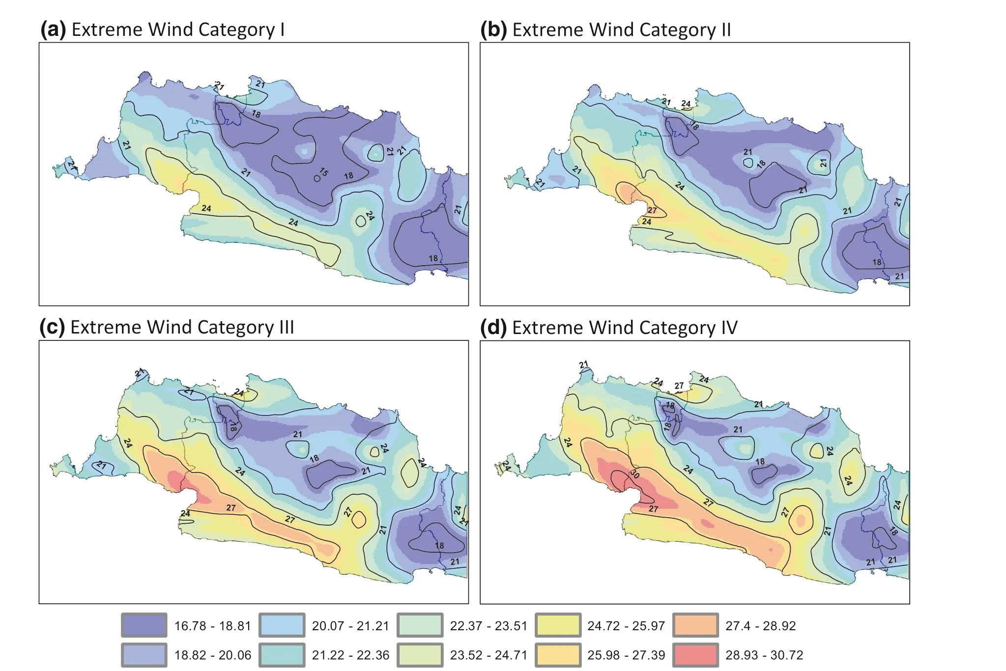
Fig. 6 Design wind speeds map (m s-1) for buildings and other structures for extreme wind categories a I (300-yr return period), b II (700-yr return period), c III (1,700-yr return period), and d IV (3,000-yr return period)
By calculating a pdf of the differences between uSand uL(Δ ≡uS-uL), we observe that the small-scale events are much more common than the large-scale events,regardless of seasons and locations(Fig.4c).Overall,about 97% of the extreme daily gust events are dominated by uScomponent.Meanwhile only 3%of the extreme gust events are attributed to higher uL.The low probability of the largescale events is consistent with Choi’s (1999) finding that extreme gusts driven by non-thunderstorm events (generally due to large-scale weather system) in Singapore were much less frequent than gusts driven by thunderstorm events (small-scale weather system). Previous studies on particular wind incidents in Indonesia frequently reported the association of wind incidents with thunderstorms (for example, Muzayanah 2015).
An interesting point is that despite the very low probability of occurrence, the large-scale-dominant wind events(Δ<0) have a normal-like distribution of u with a median of 12.2 m s-1(Fig. 4d). Meanwhile, the small-scale-dominant wind events (Δ >0) show a heavily skewed distribution of u with a smaller median of 10 m s-1.Nevertheless, the outliers of small-scale-dominant wind events are greater than the maximum of large-scale-dominant wind events (Fig. 4d).
3.3 Design Wind Speed Map and Comparison with Previous Standards
Figure 5a and b compares ERA5 wind gusts before and after the calibration. The southern coast of Java exhibits higher gust speed, which is likely caused by strong trade winds from the Indian Ocean. A striking difference is found in the inland of Java. ERA5 simulates high gust speed at 107.5°—108°E. The calibrated version, however,shows low gust speed at this region.This difference is very likely caused by the rough representation of topography in ERA5. The high gust speed appears at the top of the‘‘mountain’’ depicted in the ERA5 global model (Fig. 5a).The speed-up at the crest of the mountain is caused by compressed airflow due to increasing surface height (Stull 1988). However, a much more detailed topography map reveals a wide basin located at this location (the Bandung Basin), thus a low gust speed is dynamically expected(Fig. 5b). Concerns regarding the quality of ERA5 gust over complex topography were also mentioned in a previous study(Minola et al.2020).The validity of calibration method is also confirmed by the close resemblances of spatial variations of the calibrated data and stations data(Fig. 5b).

Fig. 7 Comparison of calculated design wind speeds with several wind loading standards, taken at high and low wind speed regions based on the new design wind map (within blue colored range). The Indonesian wind loading standards (PPPURG and SNI 1725-2016)remain constant for different return periods and different regions.The Asia-Pacific standard(HB 212-2002)does change with return period,but not with region
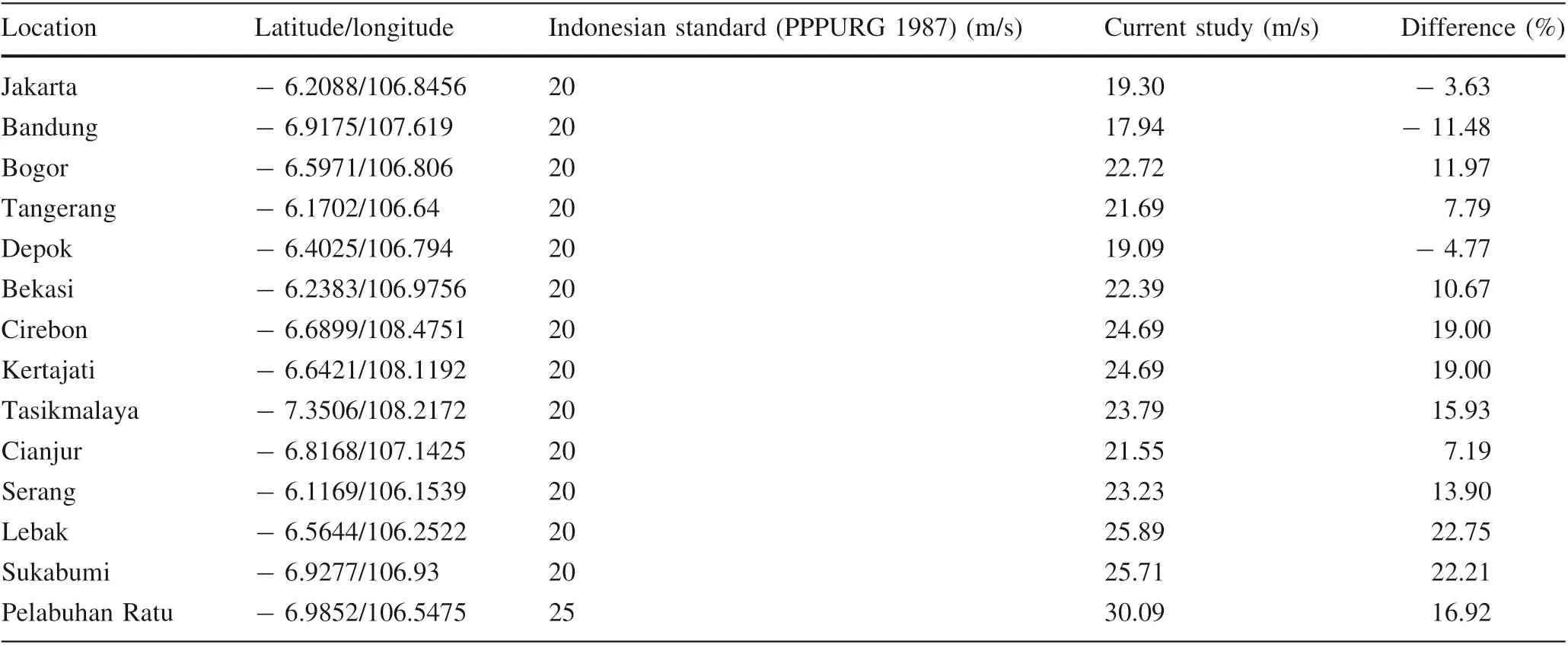
Table 2 Comparison between basic wind speed with a return period of 3,000 years (Risk Category IV) and local building standards at several grid points as representatives of some cities

Fig. 8 a Joint probability distribution functions (pdfs) of extreme wind speed category I and population density for all grid points in western Java.Horizontal and vertical dashed lines denote the medians of population density and wind speed, respectively. The percentage numbers account for the probability in each quadrant. b Spatial distribution of four risk classifications. WS wind speed, PopDen population density
The annual maxima of gust from the calibrated ERA5 are then used to calculate the design wind speed.Note that the extreme wind maps created by using mixed data or sorted data may not show much differences because of the clear dominance of a particular weather system as shown in Sect. 3.2 (Choi and Tanurdjaja 2002). Therefore, the annual maxima from different weather systems are not separated in this study. Figure 6 shows the spatial distribution of extreme wind speed in different categories following the ASCE standard.The relatively high wind speed regions are generally located in the southern part,while the northern shore has lower wind speed.This finding strongly implies that different coastal areas can experience high or low wind speeds, while the current national standards uniformly define all coastal areas as high wind speed region. The distinction solely based on inland versus coastal area as practiced by the current standards may result in either underestimated or overestimated design wind speed depending on the region. Although high wind speed regions are generally close to the southern coastal area,various inland areas also experience high wind speed,making regionally-dependent design wind speed neccessary.
Figure 7 compares the calculated design wind speed at the lowest wind speed region with that at the highest wind speed region. This value is then compared with the Australian standard, HB212-2002 Design Wind Speeds for the Asian Pacific Region (Holmes and Weller 2002), and several national standards (PPPURG and SNI 1725-2016).The HB212-2002 assigns the whole Indonesia to a design wind speed of Level 1, where the nominal wind speed is calculated by the equation of
VR=70-56R-0.1,
where R is the year return period, the consequent line is plotted in Fig. 7. This gives a value of wind speed for a 50-year return period of 32 m s-1and wind speed for a 500-yr return period of 40 m s-1.The Indonesian loading standard PPPURG assigns a general design wind speed of 20 m s-1for the whole region (considered as low wind speed) and a special speed of 25 m s-1for buildings located at all beach shorelines(considered as high wind speed).Meanwhile,the Indonesian design standard for bridges (SNI 1725-2016)assigns a horizontal design wind speed between 25 to 35 m s-1for low to high wind speed regions, although these regions are not specified on the map.
The comparison suggests that most of the Indonesian standards, which only use one design wind speed value regardless of return period, tend to yield underestimated value especially in low wind speed regions. Despite showing dependency to return period, the estimate of HB212-2002 highly overestimates the extreme wind speed for both high and low wind speed regions.Table 2 lists the design wind speed of the national standard (PPPURG) for various large cities in western Java. Some cities show less than 5% difference between the calculated design wind speed and the current standard, but other cities such as Lebak and Sukabumi show a difference as large as 20%and even higher. These differences, again, emphasize the importance of adjusting the national design wind speed standard regionally, especially to avoid underestimation in the design wind speed.
4 Discussion
Section 4.1 discusses the practical application of the new design wind map in disaster risk assessment. The limitations of this study and future research direction are discussed in Sect. 4.2.
4.1 Toward a Better Wind Disaster Risk Assessment
Although Indonesia experiences a high number of windrelated disasters every year (Sarli et al. 2020; BNPB 2021), the country currently does not have a clear wind risk map. The officials have developed an ‘‘extreme weather’’ risk map based on several hazard and vulnerability parameters as a proxy to identify areas prone to strong wind incidents (BNPB 2016). The hazard parameters were topography, land use-land cover, and annual rainfall. The use of annual rainfall was intended to describe the distribution of thunderstorms because the reported wind incidents were usually co-occurrent with heavy rainfall events (in a local term referred to as puting beliung phenomenon). However, the annual rainfall data may not be able to accurately represent thunderstorm occurrences because thunderstorms basically occur in a short period of time (30 min to hours) (Holton 2004),let alone represent the extreme wind.
To better mitigate socioeconomic impacts related to wind disasters, a more appropriate representation of extreme wind risk is needed. Our newly introduced wind map offers a potential for better risk assessment since we use a direct hazard parameter. This section demonstrates a simple risk assessment case to identify areas prone to wind disaster. The extreme wind map category I is used as the hazard component and the population density map as the vulnerability component. The population data are obtained from the Worldpop population density dataset(Gaughan et al. 2013). Figure 8a shows joint pdfs of the wind hazard and population density. Risk distributions are classified into four quadrants separated by each median in the pdfs. We found that 18.8% of western Java is exposed to a relatively high risk as denoted by stronger wind speed and higher population density. About 62.9% of the area exhibits medium risk, which indicates that the area has either stronger wind speed and lower population density, or weaker wind speed and higher population density. Meanwhile, 18.3% of the area shows a low risk due to weaker wind speed and lower population density.The spatial distribution of four risk classifications are shown in Fig. 8b.
Note that the defined risk levels are based on relative values among the categories, thus they may not measure the actual level of risks in the region of interest. Incorporating historical wind incident reports into the risk calculation is expected to improve the quality of the risk map.Furthermore, the vulnerability parameter should also consider other exposures, such as building type and building quality (Sarli et al. 2020), as well as capacity parameters related to regional economic capacity and public awareness. Moreover the new wind map can be integrated into assessments of multi-hazard analysis for spatial planning of strategic and vital infrastructures (Sakti, Rahadianto, et al.2022) and mitigation related to hydrometeorological disasters in Indonesia(Harjupa et al.2021;Sakti,Fauzi,et al.2022).
4.2 Limitations and Future Research Direction
This study is expected to benefit the stakeholders in creating a better design wind standard in western Java, and to attract more studies toward wind map development in the whole Indonesian regions. BMKG has deployed numerous AWS to all major islands of Indonesia so that a full-domain wind map hopefully could be achieved in the future.However, some notes should be taken in using the current wind map or applying the methodology.
The calibrated wind data may be sensitive to the availability of stations and topography complexity. During the interpolation of calibration coefficients in Sect. 2.2.3,errors may appear in grid boxes that are far from reference stations.Increasing availability of stations in the future will surely improve the analysis and result in a better wind map.However, building a dense meteorological station network is a great challenge that needs continuous efforts and huge investment, especially in Indonesia that consists of thousands of remote islands.To provide a confidence guideline for stakeholders, future studies may consider to carry out uncertainty analysis while performing calibration by using station data. It could be a function of distance to nearest stations and topography characteristics.
To better accommodate complex topography effects in the absence of station data, future study should consider downscaling by using a regional climate model (RCM)(Giorgi 2019) to estimate local gust characteristics. Kunz et al.(2010)successfully simulated a detailed and accurrate spatial distribution of extreme wind in Germany by using a RCM. Furthermore, the ouput of RCM could be improved by performing data assimilations of in situ or remotelysensed climate observations, resulting in a regional reanalysis (RRA) (Bollmeyer et al. 2015).
Additional care should be taken for regions that may have different climatic characteristics. For example,although Indonesia is located very close to the equator,the southernmost part of Indonesia (Lesser Sunda Islands) is sometimes directly struck by TCs (Dare et al. 2012;Mulyana et al. 2018). Design wind speed usually differentiates cases of TC and non-TC (ASCE 2017). Possible future changes of extreme wind should be anticipated because global warming has shown a significant impact on global and regional wind circulations (Vecchi and Soden 2007; Tangang et al. 2020). Exploration on other methods for design wind speed estimation may be necessary to get one with the least RMSE.
5 Conclusion
Based on observational and reanalysis wind datasets, we examined the variabilities of extreme wind and developed an extreme wind map in western Java Island. The 5-year wind observations reveal that both extreme daily mean wind and maximum wind (gust) in western Java exhibit spatial and seasonal variations. The northwestern side has higher wind speed during the northwest monsoon, and the southeastern side tends to have higher wind speed during the southeast monsoon. The time series decomposition results suggest that about 97% of extreme daily gusts are attributed to small-scale weather systems.
Incorporating the observed wind data has been proven to give added values to the local wind variation of the reanalysis, particularly in the inland area where the topography is complex.The distribution of calibrated wind speed in various areas of western Java suggests that high wind speed regions are generally located in the southern shore part of the island, while the low wind speed regions are located in the northern shore and inland. However, the Indonesian national standards fail to capture such variation as they only use one single values for the design wind speed regardless of return period and area. The national standards are likely to suffer from severe underestimation of extreme wind speed. Meanwhile, the estimate of HB212-2002 has a risk of highly overestimating the extreme wind speed. The generalization between inland versus coastal raises the concern of potential inaccuracy that varies between regions, suggesting the necessity of regional adjustment and consideration for a proper design wind speed analysis.
Acknowledgements We thank the two anonymous reviewers and the editor for their constructive comments on the early version of this article. This project was funded by the Institute of Research and Community Service, Institut Teknologi Bandung. We also thank the Java Flood One research project funded by the Newton Fund of the UKRI Natural Environment Research Council (NERC) and the Indonesian Ministry of Education and Culture for providing the additional station data.
Open AccessThis article is licensed under a Creative Commons Attribution 4.0 International License, which permits use, sharing,adaptation,distribution and reproduction in any medium or format,as long as you give appropriate credit to the original author(s) and the source,provide a link to the Creative Commons licence,and indicate if changes were made.The images or other third party material in this article are included in the article’s Creative Commons licence,unless indicated otherwise in a credit line to the material. If material is not included in the article’s Creative Commons licence and your intended use is not permitted by statutory regulation or exceeds the permitted use, you will need to obtain permission directly from the copyright holder. To view a copy of this licence, visit http://creativecommons.org/licenses/by/4.0/.
杂志排行

International Journal of Disaster Risk Science的其它文章
- A Proposed Methodological Approach for Considering Community Resilience in Technology Development and Disaster Management Pilot Testing
- The Impact of the Covid-19 Pandemic on Iranian Oil and Gas Industry Planning: A Survey of Business Continuity Challenges
- On Effective Campus Attack Response: Insights from Agent-Based Simulation for Improving Emergency Information Sharing System Design and Response Strategy
- Simulation Performance Evaluation and Uncertainty Analysis on a Coupled Inundation Model Combining SWMM and WCA2D
- Appetite for Natech Risk Information in Japan: Understanding Citizens’ Communicative Behavior Towards Risk Information Disclosure Around Osaka Bay
- Rapid Evaluation and Response to Impacts on Critical End-Use Loads Following Natural Hazard-Driven Power Outages:A Modular and Responsive Geospatial Technology