Optimized housing price prediction based on XGBoost

(University of Auckland, Auckland 999030, New Zealand)

Abstract: Objectively, housing prices are restricted by many factors and because of this, house price prediction remains a very classical and challenging problem in data analysis. In response to the redundancy of house price data, which makes it difficult to identify important features in practical scenarios, this paper proposes an innovative approach to data pre-processing and data prediction by means of double model iterative fitting. The initial data is pre-processed in terms of data meaning, data form and data relevance, then suitable models are selected for training. In traditional machine learning, Random Forest (RF) and XGBoost (XGB) are two commonly used methods. The RF model is able to accurately judge "redundant" features through its Bagging process. The XGB model, while improving prediction, is also limited by its reduced generalisation ability and cannot stably reflect the importance of features. Therefore, this paper uses the RF model to process redundant data and uses the XGB model to fit new data sets to improve the prediction results. In this paper, experiments were conducted on the Kaggle competition dataset ("House Prices-Advanced Regression Techniques") and the test results showed that the final regression accuracy R2 of the XGB regression model was 87%, while the R2 of the single RF model and the single XGB model were 79.2% and 78.7%, respectively. The experiment proves that the data prediction method can significantly improve the effect of housing price prediction. To fully reflect the model fitting effect and prediction ability, the authors change the "house price" to discrete variable which has two categories of "high" and "low", and get the Confusion Matrix with an precision of 93% and a recall of 93%.

Keywords: House price prediction； Machine learning； XGBoost； Random Forest； Iterative model regression

1 Introduction

With the growth of global population, industrialization and urbanization, housing has gradually become a very significant socio-economic issue. The demand for housing, the need for a good living environment, and the need for housing infrastructure are all increasing. Likewise, as these housing needs persist continually and lead to a growing housing price market, house providers want to meet these needs as much as possible in order to increase the expected price of housing and thus maximize their profits. Since the 21st century, home prices have not only been a key concern in any region of any country, but are influenced by many factors. Therefore, it is difficult for us to identify the most effective housing characteristics that affect the price of housing and to give a most cost-effective housing maintenance plan when the only thing we can change as a landlord is our own home.

Putting aside many other factors, such as the national housing price macro-control policies, we start from the condition of house and the surrounding environment, extracting useful information from a large amount of housing data to predict house prices more accurately. In the field of Machine Learning (ML), the house price prediction problem is a classic problem. However, the predicted house prices using machine learning methods do not address the actual needs of landlords, in other words, guaranteeing a single prediction accuracy does not provide users with enough suggestions to improve their homes and thus increase home prices.

For example,

(1) How do the results we predict using ML help end-users? In fact, ML prediction results are not user-friendly. What users need should be the methods to improve the results of ML prediction rather than the prediction results themselves.

(2) We expect that ML can calculate the feature importance in the prediction process and filter the features that are important enough for the prediction result by the feature importance. Can we obtain more effective datasets to improve the prediction effect by feature filtering? Can we reasonably explain the impact of these features on house prices?

(3) When a user wants to renovate a house, which changeable house features can be optimized to maximize the price of the house?

This study is dedicated to solve all the above problems by deploying algorithmic machine learning for house price prediction. Data processing, optimization algorithms, and feature filtering are used to improve the prediction accuracy and strengthen the prediction effect. The purpose of this thesis is to obtain a high accurate model through feature filtering and to explain the impact of important features on house prices. Finally, it provides users with suggestions that can improve housing returns, completing the transition from predicting house prices to improving them based on machine learning.

Therefore, based on machine learning, we need to not only predict house prices, but more importantly, be able to study the data at a theoretical level to build user-facing systems that can provide practical help to users in solving house price improvement problems. We intend to use machine learning to accomplish the following goals: (1) Build highly accurate models.(2) Calculate feature importance by model.(3) Make results understandable and provide recommendations to users.

To accomplish these goals, we have studied various machine learning algorithms and related techniques. Here are some brief descriptions of our approach:

(1) We use two machine learning techniques to get a high accuracy model. Firstly, we use Random Forest (RF) for regression, and get feature importance from the Random Forest Regressor. Then we filter the features based on the importance to create a new data set. Finally we build XGBoost to regress and use it to predict the house price.

(2) After obtaining a regression model with higher accuracy, we then labeled the house prices as "High" or "Low" and used the XGBoost Classifier with the selected features to provide a prediction model with at least 92% accuracy.

(3) Finally, we explain the impact of each feature on the house price category by feature importance based on the classification model and provide suggestions for users to upgrade their house price.

2 Related work

In the field of machine learning, many attempts have been made to predict house prices, such as some algorithmic machine learning: support vector machines, various clustering, and tree-based learning systems, and even brain-like machine learning, such as various types of neural networks. The following section includes the review of the relevant literature, the relevant research methods, and the relevant techniques used.

2.1 Literature review

When facing with a data analysis problem, we usually think about two questions to investigate, "What" and "How": what kind of data should we collect to support our investigation to the problem, and how to analyze the data we collect.

The data for house price ML models: We have always believed that data collection and pre-processing are the most important and time-consuming part in data analysis. During the modeling process, we can improve the results by changing the model or the parameters of the model, but if the dataset itself is not good, such improvement is minimal. Therefore, we discuss some related work about which data should use for data analysis of ML models.

(1) In previous studies, when analyzing data on housing prices, the analysis is often limited to a region because of too many uncertainties, so a model for predicting property prices[1]is proposed, which can be used universally in any region with little fine-tuning. This model reflects that some location factors, such as public/transportation facilities (office, college, super market and transportation facilityetc.), have a significant impact on house prices in a given area when predicting property prices.

(2) In one study[2], the house features that buyers are interested in (like ‘square feet area’, ‘no. of Bedrooms’, ‘no. of Bathrooms’, ‘Type of Flooring’, ‘Lift availability’) are also used as a data set for house price forecasting. In this paper, the authors use Linear, Forest, and Boosted regressions to fit this data set and improve the prediction accuracy.

(3) In previous studies, the hedonic methodology was proposed to analyze the Factors influencing the value of houses[3], in which it was argued that house prices are highly influenced by position quality and typological quality.

(4) In contrast to using a single model (e.g., a linear model) for house price prediction, the author use Hedonic Price Model and Artificial Neural Network for comparison in his study[4], not only to confirm that house characteristics and house prices do not show a linear relationship, but also to prove that in addition to factors such as environmental attributes, house characteristics themselves can significantly affect house prices.

The ML models for house price prediction: In previous studies, various machine learning methods have been used for house price prediction. We integrate papers that utilize multiple/combined machine learning algorithms for house price prediction and use the results of these related studies to identify which models might be used in our research.

(1) Four advanced regression technique were applied for this case[5], and since Decision Tree overfits the dataset collected in this study, the authors used Linear Regression, Lasso Regression, Ridge Regression and ElasticNet Regression for house price prediction, usedR2score to evaluate models, and Adjusted-R2score to indicate if the new term improves the model accuracy. The results of the study indicate Linear regression model has the best prediction effect (R2= 0.695)

(2) In previous studies[6], four machine learning algorithms, C4.5, RIPPER, Naïve Bayesian, and AdaBoost, were used to build house price prediction models for comparison experiments. The experimental results show that the RIPPER algorithm model has the best prediction effect, being able to obtain an Average test error of 0.2488, while the Average test error of AdaBoost′s method is also able to reach 0.2570.

(3) Brain-like machine learning models (e.g., neural networks) are commonly used for hard-to-fit data sets (e.g., unbalanced data sets). There have been attempts to use such an approach for research in house price prediction[7]. In this study, three different models have been formed with the Support Vector Machines (SVM), feedforward artificial neural networks (MLP) and Generalized Regression Neural Networks (GRNN), and Mean Absolute Percentage Error (MAPE) was selected as the error metric. The result shows that MLP gets the best performance with MAPE equal to 9.3% in rental listings and 14.9% for sale listings.

(4) A study provides the performance of multiple linear regression models, feedforward neural network models, and XGBoost models for house price prediction. It finds that linear regression models are under-expressed, feedforward neural networks are unstable and expensive to train. On the contrary, tree-based models perform relatively well for house price prediction. The results show that the XGBoost is superior to traditional regression models as an ensemble learning algorithm for tree-based models, whose average RMSE of training is 0.0178.

2.2 Research method

ML models have been widely used in the field of house price prediction, and tree-based ML models (e.g., random forest) can have good prediction performance when dealing with most of the house price data, but due to the uncertain number of data features, they are easily overfitted or underfitted, resulting in low generalization ability of the models. Meanwhile, most studies focus on how to improve the prediction performance and ignore the user-friendliness of the prediction results, in other words, there is no good transition from theory to practical application,i.e., users should be able to know how to improve their house prices from the results.

In the present study, we work to address the above-mentioned research gaps. The research methods flow is provided in Fig.1.

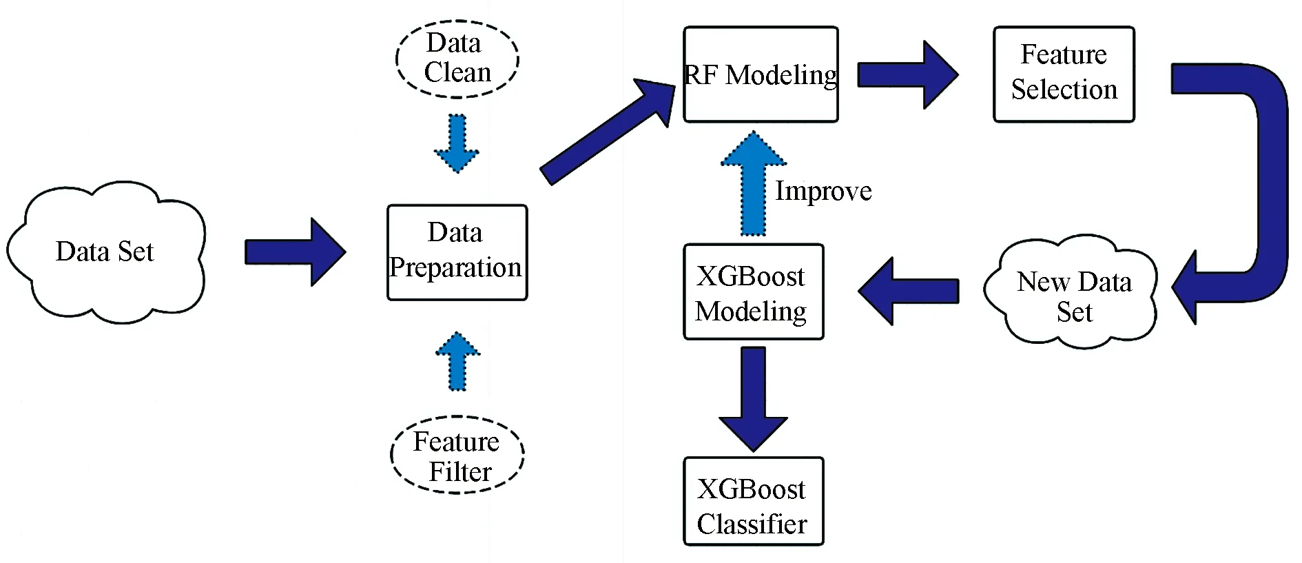
Fig.1 The research methods flow

In this research, we use the dataset from the Kaggle competition website (House Prices-Advanced Regression Techniques). RF model and XGBoost model are used for house price prediction and for feature selection, and also, to compare their prediction performance and explain the reasons.

The research methods are divided into improving house price prediction performance and interpreting house price prediction results. We use a Random Forest full model for house price prediction and feature filtering by the importance of the features obtained from the model. Then we use a new model, XGBoost (eXtreme Gradient Boosting) for improving house price prediction performance. This is proposed by Chenetal.[8], an integrated machine learning algorithm Based on Decision Trees (GBDT). And reasonable feature reduction will also enhance the generalization of the model. On the other hand, we compare the two models, explain the model principles to explain the prediction results and feature importance, and provide users with reasonable and effective suggestions to improve house prices.

3.1 Feature engineering

Data pre-processing has been considered as the core and time-consuming part of the data analysis process, which includes data observation, data filtering, data cleaning, data transformation, data format standardization,etc.In this section, we will present the data pre-processing steps performed on our data set ("house-prices-advanced-regression-techniques") in detail.

3.1.1 Data description The data set has a total of 1460 samples, each with 80 features. Some of these features are used to measure the house itself, and some are used to record the house′s surroundings.

Overall data: (1) Prediction labels: 1460*1.(2) Feature matrix: 1460*80.

Data types include: (1) Float64 (3).(2) Int64 (35).(3) Object (discrete string type) (43).

First, house features include two types, continuous features and categorical features. The data type of continuous features is float64, while the data type of categorical features is more complex, including int64 and discrete string types.

3.1.2 Data cleaning

(1) Feature dropping. When preparing the data, we should know the source of the data and comprehend the meaning of the features. Because there is often some data that can be determined to be dropped before modeling without losing any information.

(a) Mark data & same information data.‘Id’ column just use for marking each house, so it looks like this feature doesn′t help our modeling. ‘Year Built’ and ‘Year Remod Add’ column seems to give the same information for us. ‘YearBuilt’ is used to record the original construction date, and ‘YearRemodAdd’ means the remodel date which same as construction date if no remodeling or additions. So we can drop ‘Id’ and ‘Year Built’.

(b) "Sparse" data. We call the feature with too many same values as "Sparse" data, and we still need to determine whether it can be dropped or not from the meaning of the feature. We list some of the features that have more than 90% of the same values in the total sample below.

(i) Features with too many duplicate values

‘Street’, ‘Alley’, ‘Utilities’, ‘LandSlope’,etc.

(ii) Features with too many NaN value

‘PoolQC’, ‘MiscFeature’.

Although special value can have a significant impact on house prices when instances generally have same feature values, we do not believe that the above two types of features can be the key to fitting house prices when they are generally consistent (we may even refer to the special value as "outliers"), so we left no features of those "sparse" data.

(2) Missing values. We have divided the missing values into two categories, one part of them is missing completely at random, called MCAR missing values, and the other part comes from human records. We discuss the handling of these two missing values separately.

(a) Artificially recorded values as ‘NaN’.There are many categorical feature values that are artificially recorded as "NA", which are used to represent the category "None". For example, ‘Garage Qual’ means Garage quality, whose missing value "NA" stands for those houses without Garage, but such records are treated as missing values by the model. Therefore, we replace the missing values with "None" for these categories.

(b) MCAR missing values. Due to the reasons like simple data distribution, we choose to use some common missing value imputation methods. For continuous features, we use the mean fill null values, and in the case of categorical features, we use the most frequently class to fill the missing values.

(3) Data transformation.

(a) Categorical features.There are many encoding methods available, but we only consider hard encoding and one-hot encoding. Hard encoding maps category features to numerical values, which coincide with the number of categories. Hot-Encoding is commonly used for discrete and out of order data due to its unique one-bit valid encoding property.

In fact, there are many categorical features in our data have clear sequential relationships,e.g., in the ‘Exter Qual’ column ("Evaluates the quality of the material on the exterior") we have five value to represent five level of the the quality: "Excellent", "Good", "Average/Typical", "Fair", "Poor".

Also, hard encoding can effectively buffer the effect of numerical categories on the values,e.g., ‘MSSub Class’ column has a class represented by the value 190, which must have a huge impact on the model, hard encoding can encode it as 16 thus reducing the impact.

Finally, since there are discrete features with many categories in the data set, we do not have enough space to store such huge sparse data,e.g., ‘Exterior 2nd’ has 17 categories, which means we need more than 17 columns of sparse matrix to replace this one feature. So we finally choose to use hard coding, and since we are encoding the features rather than the target, we use the OrdinalEcnoder in the "Scikit-learn" package.

(b) Continuous features.Continuous features are also multidimensional, and obviously, the scale of these features and the magnitude of the values are different (e.g., ‘BedroomAbvGr’ records the number of bedrooms above grade, while ‘1stFlrSF’ records first floor square feet), then they will have different degrees of influence on house prices. By standardization, it is possible to make different features have the same scale.

We use the StandardScaler in the "Scikit-learn" package to normalize the data distribution to a distribution with a mean of 0 and a variance of 1, using the following formula (1).

(1)

Where theμmeans the mean of feature, andσmeans the standard deviation of feature.

By the way, although the decision tree model does not need to be normalized, we still standardize the continuous features because of the gradient boosting property of XGBoost.

3.1.3 Response variables normalization When we focus on cleaning feature variables in our data preparation, we often ignore the response variables. In tree-based machine learning prediction, we prefer not to treat the response variables. This is because some pre-processing like StandardScaler for the response variables would lead to distorted data and unintelligible forecasts (e.g., negative house price forecasts).

Although dealing with response variables may raise data analysis problems, we still need to make judgments about the data distribution of response variables. Because if response variable data is not normally distributed, it will affect the results of regression analysis (most obvious for linear regression). There are many statistical tests for normality, such as the Kolmogorov-Smirnov test (K-S test), the Shapiro-Wilk test (S-W test), and theχ2Goodness-of-fit test[8]. In our study, the method of plotting frequency distribution histograms is used to test the data distribution in order to make possible subsequent data transformations more convenient.

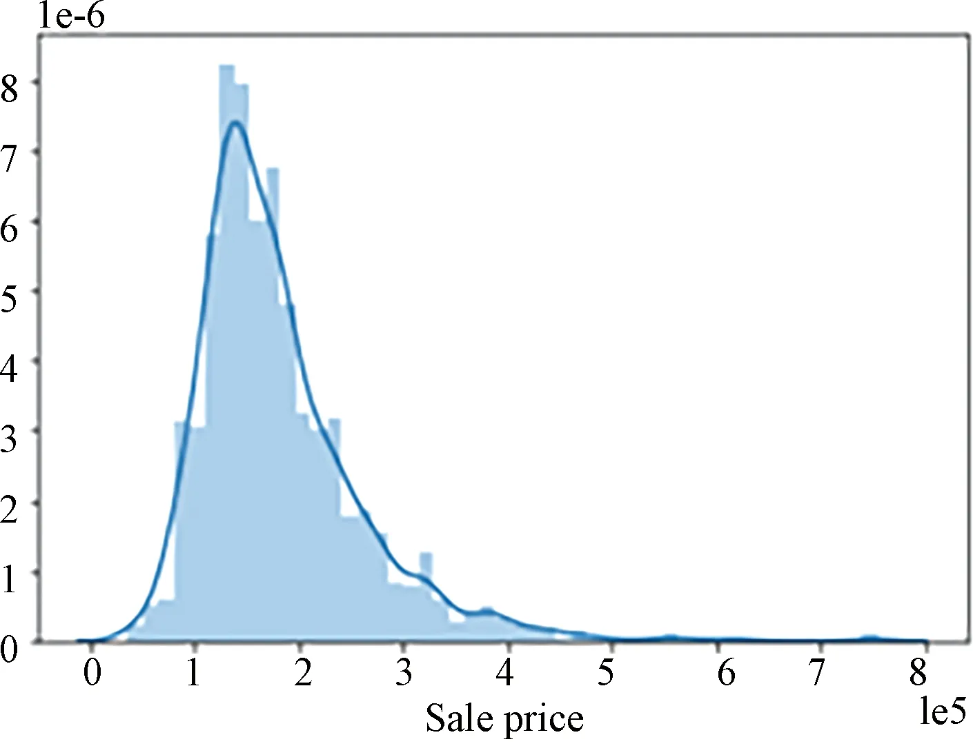
Fig.2 Original data distribution chart

In the Fig.2, the distribution of response variables is found to be right skewed by plotting, which has a huge impact on the prediction accuracy. Even for a tree-based model, such response variables would affect the results of the regression analysis.

A right skewed distribution means that the mean of the data is larger than the plurality, in other words, there are a few values that are particularly large, and we need to minimize the gap between the data. So we choose to use the logarithmic transformation (2)

Yscaled=log(Y)

(2)

to deal with the response variable, and Fig.3 gives the distribution of the transformed response variable data.

3.1.4 Feature correlation After the data encoding and normalization, we need to consider the last issue, which is feature correlation. When measuring data based on relevance, usually a feature is considered good when it has a strong relationship with the label and a low relevance with other features[9]. This is because features with high correlation could get many statistical problems when used to fit a model (e.g., multicollinearity, information redundancy,etc.), which can lead to a poor fit.

In the case where the correlation coefficient is between -1 to 1 (a negative number is an inverse correlation and a positive number is a positive correlation), we define a pair of features as highly correlated with absolute value of correlation exceeding 0.7, and drop one of them by their correlation with the response variables.

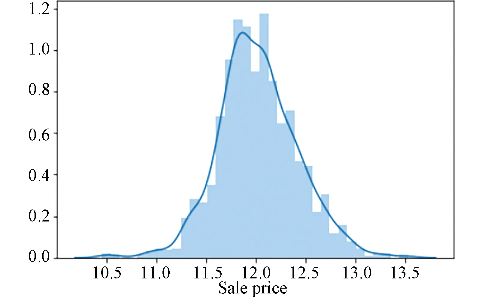
Fig.3 Transformed data distribution chart

(1) Continuous features. For continuous features, since we have previously transformed them into normal distributions by normalization, and we are more concerned with the linear relationship between them, we evaluate these features using the Pearson correlation coefficient (3), the formula as follows[10]:

(3)

Whereρa,bmeans the Pearson correlation coefficient between featureaandb;E(ab) is the cross-correlation betweenaandb; andσmeans standard deviation.

By calculating the Pearson correlation coefficient, Tab.1 lists the features with absolute values above 0.7, which are considered highly correlated.

Now we need to decide which features to drop, and in Tab.2 the Pearson correlation coefficients of the above features with the response variables ‘SalePrice’ are given.

Tab.1 The Pearson correlation coefficient table

Tab.2 The Pearson correlation coefficient with ‘SalePrice’

From Tab.1 and Tab.2, we decide to keep ‘YearBuilt’ and ‘TotalBsmtSF’ columns.

(2) Categorical features. When evaluating Categorical feature correlations, we are interested in those features with sequential category (ratings of housing status,etc.), because there is no explicit relationship between unordered categorical variables. Therefore, we use the Kendall correlation coefficient[11]to evaluate the degree of correlation between ordinal categorical features. The following is the formula for the Kendall correlation coefficient (4).

(4)

WhereτX1,X2means the Kendall correlation coefficient between featureX1andX2;p1means the ordered pairs that compose the ordered set;dΔ(p1,p2) means the symmetric difference distance betweenp1andp2(for example;pis [a,b],[a,c],[b,c] for a ordered set [a,b,c]; anddΔis length of [b,c],[c,b] forp{[a,b],[a,c],[b,c] andp{[a,b],[a,c],[c,b]);Nmeans the length of ordered set (usually features with ordered sets of the same length are likely to be considered as highly correlated).

Tab.3 The Kendall correlation coefficient table

By calculating the Kendall correlation coefficient, Tab.3 lists the features with absolute values above 0.7, which are considered highly correlated.

We do not use the Kendall correlation coefficient when calculating the correlation coefficient between the above features and the response variable ‘SalePrice’. ‘SalePrice’ is a continuous column with normal distribution, while the above features are discrete without normalization, so we choose to use the Spearman correlation coefficient. The following is the Spearman correlation coefficient formula (5).

(5)

The Spearman correlation coefficient is calculated in the same manner as Equation (3), except thatρar,bris calculated after bothaandbhave been rank transformed to values between 1 andN(arandbr),Nis the number of samples. And a so-called fractional ranking is used, which means that the mean rank is assigned in case of ties[12].

Then we use the Spearman correlation coefficient to decide which feature should be keep, and in Tab.4 the Spearman correlation coefficients of the features in Tab.3 with the response variables ‘SalePrice’ are given.

Tab.4 The Spearman correlation coefficient with ‘SalePrice’

So from Tab.3 and Tab.4, we decide to drop ‘Exterior1st’ and ‘GarageQual’ features.

3.2 Random forest regression

Random forest is a combination of tree predictors such that each tree depends on the values of a random vector that are sampled independently and have the same distribution for all trees in the forest[13]. In simple terms, random forest uses the idea of bagging to create reasonable randomness, and combines multiple CART decision tree weak learners to obtain their respective prediction results, and makes the final results with high accuracy and generalization performance by integration. For classification problems, the final category is obtained as the output using the voting method, and for regression problems, the final prediction is obtained as the model output using aggregation (e.g., taking the arithmetic mean,etc.)

Fig.4 provides the flow of data analysis using random forest. After completing the modeling, feature importance is obtained for subsequent feature selection.

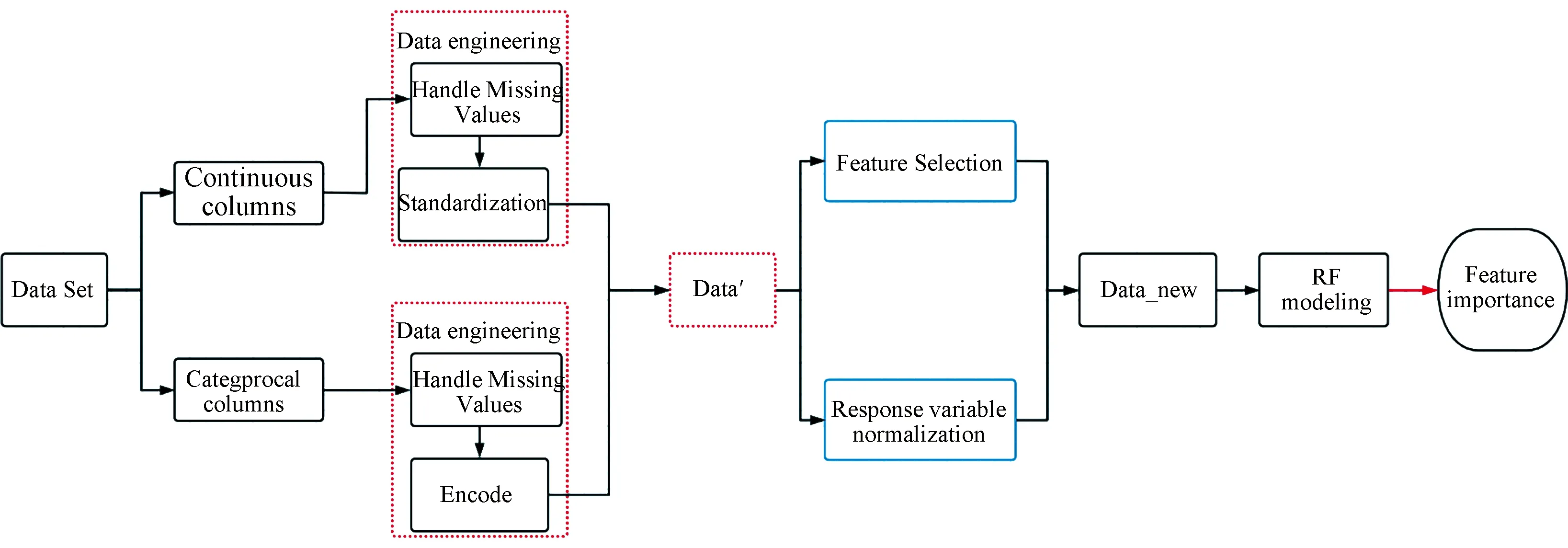
Fig. 4 The Random Forest modeling flow

3.2.1 Data preprocessing Random forest as our prior model is mainly used to explore the data, and in this case, the overall information of the data is unknown. Therefore, the data used in the RF model should be processed by the above mentioned feature engineering to make it valid.

(1) The data pre-processing process is divided into continuous variables processing and discrete variables processing:

(a) Continuous variables processing.

From Fig.5, we can see that there are missing values in the continuous columns, we use the SimpleImputer with strategy of calculating the mean value to estimate missing value, and then normalize all continuous data to satisfy normal distribution by StandardScaler.

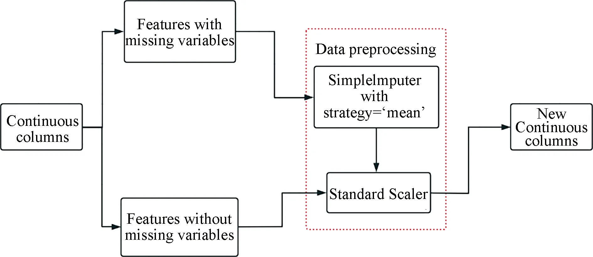
Fig.5 Continuous variables processing pipeline

(b) Discrete variables processing.

In Fig.6, since categorical variables have have two types of missing values, artificially recorded "NaN" and MCAR missing values, we choose two strategies of SimpleImputer, which are getting imputed with the most frequent term and the constant term "None". Then we use OrdinalEncoder with "dtype=np.int" to encode discrete values into integers.

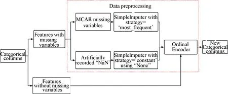
Fig.6 Discrete variables processing pipeline

(2) After processing the data into a legal form for the ML model, we filtered the features by understanding the meaning of each feature itself (mentioned in 3.1.2(1)Feature Dropping), defining the "Sparse" data and calculating the correlation coefficients, the pipeline is given in Fig.7.

Fig.7 The features selection flow

Then we provide a new data set Datanewfor fitting the model. The number of features, the sample size of Datanewand the conversion of response variables are given in Tab.5.

Tab.5 The Dat anew Structure

(3) In each random sampling round of Bagging, a portion of the training set that is not sampled is called Out Of Bag (OOB for short). In fact, the optimal sample size of OOB in Bagging is always 20% or 40%, which allows the combined model to exhibit a good overall performance[14]. These OOBs are not involved in the fitting of the training set model, so they can be used to check the generalization ability of the model. Similarly, we randomly divide Datanewinto a training set and a validation set in the ratio of 7∶3, with the training set used to fit the model and the validation set used to evaluate the model fit.

3.2.2 Modeling After completing the data engineering, modeling is actually very simple. When our data is good enough, the prediction will not be very bad. There is a limit to the information in the data, we build the model and tune the parameters to approximate that limit.

First, we fit the regression model and set up the entire random forest architecture with the following four more important parameters.

(1) ‘n_estimators’: The number of sub-datasets generated from the original data set with replacement sampling,i.e., the number of decision trees.

(2) ‘max_features’: The maximum number of features allowed in Random forest on a single decision tree. It has several types of options available.

(3) ‘max_samples’: The maximum number of random samples that can be used to construct the tree in each iteration.

(4) ‘criterion’: The calculation method used to determine whether the node continues to split,i.e., the performance evaluation criteria.

We use cross-validation to set parameters, and since the optimal parameters are unknown, two cross-validation-based parameter search methods are derived, Grid Search and Randomized Search. GridSearchCV sequentially adjusts the parameters in steps within the specified parameter range, and uses the adjusted parameters to train the learner to find the parameter with the highest accuracy on the validation set from all the parameters. RandomizedSearchCV actually uses the same approach as GridSearchCV, but it replaces GridSearchCV′s grid search for parameters with random sampling in the parameter space. Our data quality is relatively good, so the number of parameters to be set in the modeling is small, and the data set is small, so grid search is chosen.

The optimal parameters of the model are given in Tab.6.

Tab.6 The optimal parameters of RF regressor

3.2.3 Regression effect evaluation For regression models, there are many evaluation indicators, such as Mean Absolute Error (MAE), which is used to reflect the actual situation of the prediction value error, and Mean Squared Error (MSE), which can evaluate the degree of data variation. The smaller the MSE value, the better the model can describe the experimental data.

Since we predict the result as log(‘Sale Price’), the predicted house price can be viewed by exp(‘Sale Price’). When we evaluate the model by the above two forms of response variables, the values of both MAE and MSE will change significantly. In order to meet our requirements for the prediction results, we choose to use theR2coefficient of determination to evaluate the regression model, following is the formula (6) for theR2coefficient of determination:

(6)

From the formula, the denominator is understood as the degree of dispersion of the original data, the numerator is the error between the predicted data and the original data, and the division of the two can eliminate the influence of the degree of dispersion of the original data. In fact, the "coefficient of determination" describes the goodness of fit by the change of data. Theoretical value range(-∞,1], normal value range is [0,1] (the negative coefficient of determination implies that the prediction is even less effective than taking the mean value). The closerR2is to 1, the stronger the model′s ability to explain the response variable.

The Random Forest model we use has anR2of 85%.

3.2.4 Feature importance One of the features of the integrated learning model is that it can output feature importance, which can assist us in filtering features, thus making the model more robust.

The idea of performing feature importance evaluation in random forest is determine how much each feature contributes to each tree in the random forest, then take an average value, and finally compare the contribution size among the features, where the calculation regarding the contribution can be either impurity or out-of-bag data error (OOB error)[15].

(1) Based on OOB error.

For a tree, out-of-bag data errors can reflect the generalization ability of the learner. When we calculate the importance of featureX, we calculate itsOOBerror1from the out-of-bag data of each tree, and then add noise interference to theXfeature to calculate theOOBerror2at this time, assuming there are N trees, then the importance of theXfeature is 1/N×∑(OOBerror2-OOBerror1).

The reason why this value can indicate the importance of the feature is that if the out-of-bag data accuracy decreases substantially after adding random noise (i.e.,OOBerror2rises), indicating that this feature has a large impact on the prediction results of the sample, which in turn indicates a relatively high degree of importance.

(2) Based on impurity.

Each node in a decision tree is segmented by a feature, and the nodes can be identified using impurity,i.e., when training a decision tree, it is possible to calculate how much of the tree′s impurity the feature reduces. For a decision tree forest, it is possible to calculate how much impurity each feature reduces on average, and use its average reduction in impurity as a basis for feature importance.

For the regression model, the impurity we use is MSE (Mean Square Error) (7).

(7)

We calculate the random forest feature importance to provide a better data set for the XGBoost model that follows, so we choose to use impurity-based feature importance, which is more convenient, to identify the more important features. Tab.7 provides the importance of the top five important features calculated from the random forest.

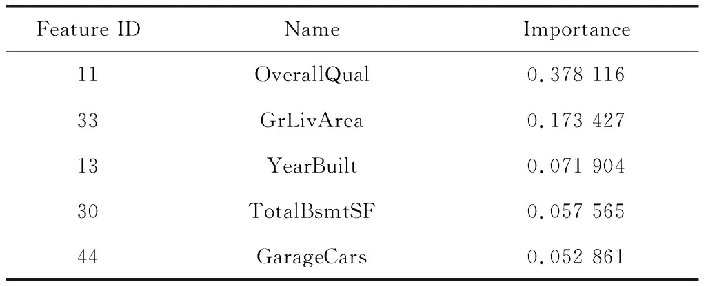
Tab.7 The top-5 random forest importance of feature

3.3 XGBoost regression

XGBoost is a scalable machine learning system for tree boosting. Boosting is an iterative algorithm where each iteration weights the samples according to the prediction results of the previous iteration, and as the iterations continue, the error gets smaller and the bias of the model decreases[8].In simple terms, XGBoost uses this idea to reduce bias by using an architecture-fixed model that is fitted on the basis of the residuals (the difference between the last prediction and the true result) from the last tree fit.

We use the XGBoost model to fit the new data set created by the random forest model above as a way to improve the prediction.

Fig.8 provides the flow of data analysis using XGBoost. We will analyze feature importance after completing the modeling.

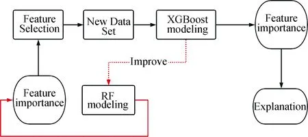
Fig.8 The XGBoost modeling flow

3.3.1 New data set building From the feature importance of the random forest, it can be seen that the ‘OverallQual’ feature is much more important than the other features, mainly because we chose to use the impurity-based assessment of feature importance. In the feature selection based on impurity reduction, when a feature is selected, the importance of other features associated with it becomes low, because the impurity they can reduce is removed when the feature is selected.

‘OverallQual’ means ‘Rates the overall material and finish of the house’. Obviously there will be many features associated with ‘OverallQual’, so although the importance of other features seems low, we still choose the top-30 most important features to form the new data set. Tab.8 provides the structure of the data set used for the XGBoost.

Tab.8 The datase tnew Structure

3.3.2 Modeling When we modeling with XGBoost regressor, we also need to set some important hyperparameters.

(1) ‘n_estimators’: Same as ‘num_boosting_rounds’, which means the number of boosting iterations,i.e.how many base models are generated.

(2) ‘max_depth’: This value is the maximum depth of the tree used to avoid overfitting.

(3) ‘learning_rate’: Same as ‘eta’. The shrinkage step used in the boosting process in order to prevent overfitting.

(4) ‘objective’: This parameter defines the loss function that needs to be minimized.

Similarly, we use GridSearchCV to find the optimal parameters. The optimal parameters of the model are given in Tab.9.

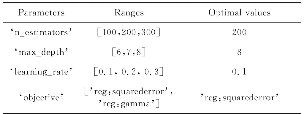
Tab.9 The optimal parameters of XGB regressor

3.3.3 Regression effect evaluation In terms of regression prediction, the XGboost model outperforms the Random Forest model, the details of which are provided in Tab.10.

Tab.10 Comparison of regression fitting effects

3.3.4 Feature importance The XGBoost regression model does not calculate the importance of features in the same way as Random Forest. Overall, the importance is expressed using the proportion of the feature score to total feature scores, with the following formula (8).

(8)

Wherescoreis the list of each feature importance score; and sum(score) means the total feature scores. We can see that this calculation is able to avoid the problem of features interacting with each other and forcing some features to become less important. But again, we are faced with another problem, what to use to represent the feature importance score. Three common ways of doing this are given below.

(1) weight: The number of times a feature is used to split the data across all trees.

(2) cover: The average coverage across all splits the feature is used in. Thetotal_coverof a feature is the total number of samples split by the feature, socoveristotal_cover/weight.

(3) gain: The average gain across all splits the feature is used in. Thetotal_gainmeans the total gain brought about by a feature at each splitting of node in all trees, sogainistotal_gain/weight.

In most cases, gain is the most relevant attribute to explain the importance of each feature, so we have also chosen to use gain to reflect feature importance. Here is the formula for calculating Gain for the XGBoost model (9).

(9)

To refine, the second order Taylor expansion used to approximate the XGBoost loss function has two coefficients, the first and second order gradient statistics on the last loss function, denoted asgiandhi. "the last loss function" means thatgiandhiare known at the time we train the current tree. Assume thatILandIRare the instance sets of left and right nodes after the split. LetI=IL∪IR, then for example,GL=∑i∈ILgiandHL=∑i∈ILhi.

Tab.11 provides the Gain-based feature importance of the top ten important features of XGBoost Regressor.

3.3.5 Feature analysis It is clear that the feature importance rank of the XGB regression model is very different from that of the RF regression model.

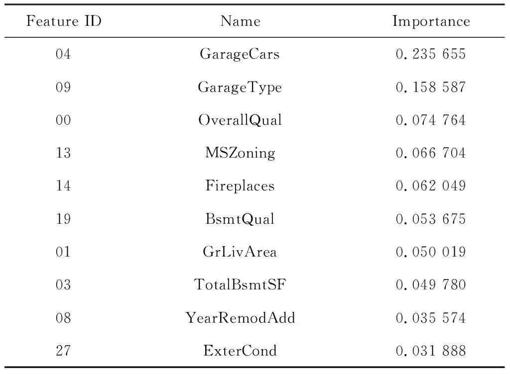
Tab.11 The top-10 XGBoost importance of feature

In the RF regression model, ‘OverallQual’ as the most important feature dominates all other features. The reason for this is related to the way feature importance is calculated in the RF model. As mentioned earlier, there are several points to note when ranking feature importance based on impurity.

(1) Feature importance based on reduced impurity will tend to select features with more categories (such features are more likely to appear in the nodes of the decision tree).

(2) When there are related features, the importance of other features that are related to a feature becomes low after the first feature has been selected (because the impurity they can reduce has been removed by the previous features).

In the XGB regression model,Gainis not only used to evaluate feature importance, but is also used in a pre-pruning strategy (only splitting ifGainis greater than 0 after splitting). Such a calculation avoids the problems encountered in RF regression models and also allows for a quantitative description of feature importance.

In the XGB regression model with anR2score of 87%, the most important feature is the garage information,

(a) ‘GarageCars’: Size of garage in car capacity.

(b) ‘GarageType’: Garage location with 7 classes.

which seems reasonable, as people buying a house always think about the convenience of parking. It is to be expected that the assessments of house influence the price of the house to a large extent,

(a) ‘BsmtQual’: Evaluates the height of the basement with 6 classes.

(b) ‘OverallQual’: Rates the overall material and finish of the house with 10 classes.

But for the moment, these are the ‘attributes’ that affect house prices and it is difficult for landlords to change them. So I find some changeable features and documented them to help with Actionability later,

(a) ‘ExterQual’: Evaluates the quality of the material on the exterior with 5 classes.

(b) ‘ExterCond’: Evaluates the present condition of the material on the exterior with 5 classes.

(c) ‘BsmtFinType1’: Rating of basement finished area with 7 classes.

(d) ‘BsmtFinSF1’: Type 1 finished square feet.

4 From explainability to actionability

We have succeeded in improving house price prediction by creating a new dataset and using the XGBoost model, while gaining information about the data and the features that can be interpreted to influence house prices.

Now we move from research back to theory to explain why the XGBoost regression model is better in terms of algorithmic principles. Then we turn theory to practical application.

As mentioned before, what landlords want most is not to predict how much their homes will sell for, but to know where their homes are in the overall house price market and in what way they can increase their house price levels. So we transform the regression problem into a classification problem for solving real-world problem.

4.1 Theoretical explanation

We have already briefly introduced random forests using the Bagging (bootstrap aggregating) method to build multiple decision tree models and combine them to obtain strong learners, and there are now mathematical inferences proving the convergence of random forests in some cases[16]. It is also due to convergence that the value of the loss function of the model will no longer change when the random forest is large enough[13]. We have studied the principles of XGBoost in more depth, and we are more interested in why XGBoost performs better than Random Forest.

4.1.1 XGBoost Unlike the idea of Bagging used in Random Forest, the training set does not change in each iteration of Boosting, only the weight of each sample in the learner will change accroding to the fit results of the previous iteration. The Gradient Boosted Tree uses this idea to optimise the model by reducing the loss functionLoss(F(x),y) at each iteration. XGBoost improves on the Gradient Boosted Tree to achieve a significant improvement in prediction performance.

(1) Gradient Boosted Decision Tree (GBDT) is finding a new fit label for the new base model (the negative gradient of the previous additive model), for example using the new model to fit the residuals of the previous model fit as we mentioned before. And xgboost is finding a new objective function for the new base model (second order Taylor expansion of the objective function about the new base model).

(2) XGBoost adds a penalty term for the complexity of the tree structure to the objective function to avoid overfitting and facilitate the model to obtain lower variance.

(3)…

In the following we describe in detail the principle of the XGBoost algorithm.

(10)

(b) For supervised learning, we need to define the objective function to ensure that the model learns in the right direction,i.e., the model addsK-th tree (fk) in order to make the following objective smaller:

(11)

From formula (10) and (11), we can get the objective function fork-th tree:

(12)

(13)

We analyse the above objective function (13) in two parts.

(i) Loss function.

This loss function is very complex and we use the Taylor second order expansion to approximate this function.

f(x+Δx)≈f(x)+f′(x)·Δx+

(14)

(15)

(16)

(ii) Parameterisationfk(Xi) & Ω(fk):

For the complexity of a tree, we consider that it can be expressed in terms of the number of leaf nodes and the value of the leaf nodes,

(17)

WhereTmeans the number of leaf nodes andwjis the weight of leafj.fk(Xi) refers to the prediction of thek-th tree for thei-th sample. In other word, the node which the prediction of thei-th sample falls on, so we setq(xi) to represent the location of this node.So, from function (16) and (17), we setIj={i|q(xi)=j}, then we can get the final objective function:

(18)

WhereGjis ∑i∈Ijgi; Hjis ∑i∈Ijhi.

4.1.2 Comparison between XGBoost and random forest The random forest model can be proved to be convergent using the large number theorem[16]. This means that when the number of trees is large enough, the value of the objective function of the random forest will no longer change. Due to its random nature and the underlying idea of Bagging, Random Forest focuses on reducing variance, which makes the model more generalisable but less accurate.

Boosting, on the contrary, makes the model fit better and better over iterations, but ignores the problem of overfitting when reducing bias,i.e.the model is less generalised and more accurate. However, from the XGBoost objective function (18), XGBoost adds a model complexity penalty term to avoid over-fitting while improving accuracy. This is the reason why the XGBoost model performs better than the Random Forest model.

4.2 Actionability

As mentioned earlier, we transform the regression problem into a classification problem, improving the fit while allowing the predictions to handle real-world problems.

4.2.1 Change response variables We divided the response variable into ‘high house price’ (class 1) and ‘low house price’ (class 0) by the median of ‘SalePrice’, and Fig.9 provides the data distribution transformation. The reason we use the median as the threshold between ‘high’ and ‘low house price’ here is to ensure a good fit. The median means that we will get balanced data which is more suitable for traditional supervised learning (If the data is unbalanced, the model may be biased towards large samples in the learning process and the fit will be good for large samples but poor for small samples).

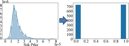
Fig.9 The data transformation flow

4.2.2 Modeling

(1) Adjustment parameters.I selected four parameters to optimize the XGboost classifier, ‘eval_metric’ indicates the evaluation function, which is used to assess the effectiveness of the model after training.

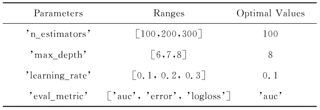
Tab.12 The optimal parameters of XGB classifier

Tab.12 gives the best parameters we have calculated by using GridSearchCV.

(2) Reset thresholds. When we use the XGB classifier for binary prediction, the model actually uses logistic regression to predict the classification probabilities and classify samples with probabilities greater than a threshold with default value 0.5 as class 1 and those less than the threshold as class 0. And we can reset the threshold to ensure that both the accuracy and recall of the model can be optimal.

Fig.10 provides the optimal threshold for the XGBoost classifier.

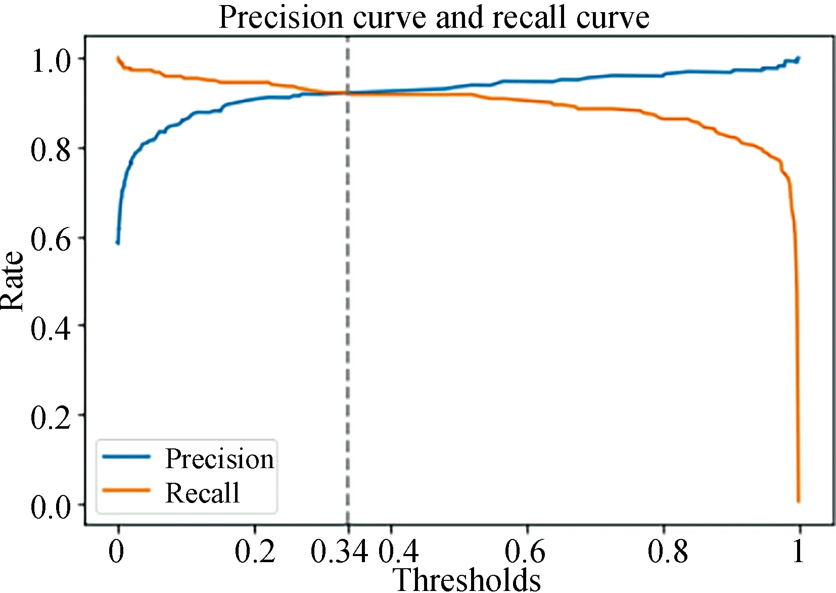
Fig.10 The best threshold

(3) Predicted effects. This XGBoost classification model has an accuracy of 93% and a recall of 93%, and Tab.13 gives details of how well the model fits.Where ‘f1score’ is the callback average of precision and recall, and ‘support’ is the number of samples in each classification.

Tab.13 The classification effects of XGB classifier

Meanwhile, the confusion matrix of the model is given in Tab.14.

Tab.14 The confusion matrix of XGB classifier

4.2.3 Feature importance Fig.11 provides theFScore-based feature importance of XGBoost Classifier. These features appear to be more evenly distributed in importance and are not influenced by other features.

Recommendations: From Fig.11 and Tab.11, we found some important and changeable features:

(a) ‘BsmtUnfSF’: Unfinished square feet of basement area

(b) ‘BsmtFinType1’: Rating of basement finished area

(c) ‘BsmtFinSF1’: Type 1 finished square feet

(d) ‘WoodDeckSF’: Wood deck area in square feet

(e) ‘MasVnrArea’: Masonry veneer area in square feet

From these features, it is clear that landlords need to improve the basement, and the exterior of the house by some way like more use of Wood deck and Masonry veneer, in order to achieve a higher price.

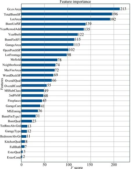
Fig.11 The XGBoost classifier feature importance

5 Conclusion and future work

There is currently a lot of research using machine learning for house price prediction. However, most of them are used to compare the performance of different ML models or just to make predictions on house prices, and have no practical use. In our study, two ML models, Random Forest and XGBoost, are combined to optimise the data fitting.

In this study, the house data ("House Prices-Advanced Regression Techniques") is obtained through the Kaggle competition and performed a complete data analysis. The dataset is cleaned in data pre-processing by data comprehension, feature correlation coefficients and so on. Then the data information is initially explored using a random forest model. And filtering features by their importance to remove redundant and useless information. Then we can provide a dataset for the XGBoost model with the potential for increased generalisation.

After fitting the XGBoost regression model, we successfully increased theR2score from 85% to 87%. At the same time, the advantages of XGBoost are explained by examining its principles. Finally, the regression problem is transformed into a classification problem to provide landlords with some suggestions to improve their house price level. In the final XGBoost classifier, we obtained a classification model with an accuracy of 93% and a recall of 93%.

There is still a lot of room for improvement in this paper,

(1) Firstly, after completing the ML classifier learning, we have only provided the user with insufficiently clear recommendations by feature importance, we need to look at the distribution of those features in data and give more specific recommendations.

(2) Our recommendations are only overall and are not able to be used for individual users. We need to build a recommendation system which, after obtaining information about a user′s home, the system is able to predict house price levels and provide targeted recommendations at the same time.

(3) Too little research has been done on the classification problem. In this study, we only used binary classification (two classes) to classify the data. We need to refine the categories and build a multi-category model.

(4) As there are likely to get a unbalanced dataset when the number of classes becomes large, because there may be some classes with only a few samples, we have to continue our research into machine learning algorithms to find solutions to poor quality datasets.

The above work can continue to improve the process of transformation from theoretical research to practical applications, make the system be able to cope with more types of data and provide users with more user-friendly features to solve practical problems. Therefore, the content of the appeal is key to our future work.