On dynamic analysis method for large-scale train-track-substructure interaction

Lei Xu

Abstract Train–track–substructure dynamic interaction is an extension of the vehicle–track coupled dynamics.It contributes to evaluate dynamic interaction and performance between train–track system and its substructures.For the first time,this work devotes to presenting engineering practical methods for modeling and solving such large-scale train–track–substructure interaction systems from a unified viewpoint.In this study,a train consists of several multi-rigid-body vehicles,and the track is modeled by various finite elements.The track length needs only satisfy the length of a train plus boundary length at two sides,despite how long the train moves on the track.The substructures and their interaction matrices to the upper track are established as independent modules,with no need for additionally building the track structures above substructures,and accordingly saving computational cost.Track–substructure local coordinates are defined to assist the confirming of the overlapped portions between the train–track system and the substructural system to effectively combine the cyclic calculation and iterative solution procedures.The advancement of this model lies in its convenience,efficiency and accuracy in continuously considering the vibration participation of multi-types of substructures against the moving of a train on the track.Numerical examples have shown the effectiveness of this method;besides,influence of substructures on train–track dynamic behaviors is illustrated accompanied by clarifying excitation difference of different track irregularity spectrums.

Keywords Train ·Track dynamic interaction ·Railway substructures ·Finite elements ·Dynamics system ·Iterative solution ·Tunnel ·Bridge

1 Introduction

1.1 Research background

In a rail transit system,the main body includes the train and its upper pantograph catenary system of power supply and lower rail infrastructural system of supporting and guidance.From aspects of civil engineering,one of the mostly concerned issue is analyzing the dynamic interaction between the train and its infrastructural system including the tracks and substructures,e.g.,the tunnel and bridge,since train–track–substructure (TTS) interaction is associated with very important railway engineering problems such as the evaluation of train running safety and riding comfort [1–3],prediction of structural fatigue damage and vibration noise[4]and revealing the mechanism of wheel–rail contact [5,6].

To evaluate the TTS interaction,computer modeling of the TTS system seems to be the most economic and practical way except the basic experimental work.As a typically large and complex system,the train,the tracks,and the substructures are expected to be elaborated sophisticatedly to accurately depict the system’s dynamic behaviors,but sometimes making a compromise to efficiency.Generally,two categories of analytical and numerical methods are adopted to the TTS dynamics,but the analytical method can be merely suitable for very simplified structures with moving constant,pulsating or continuous forces with constant speed [7,8],and accordingly,the most research nowadays concentrates on numerical methods.

1.2 State-of-the-art review

In conventional research,an emphasis is mainly put on train–bridge interaction where the detailed configuration of track structure is neglected,for more than one hundred years.Yang and Yau [9] presented a vehicle–bridge element to accurately and efficiently modeling and analyzing the vehicle–bridge interaction.Xia and Zhang [10,11]established representative vehicle–bridge interaction models:one is built in global equations with time-dependent coefficients and the other is solved by an inter-system iteration method.Iterative methods has also been applied by scholars in a series of work,such as Feriani et al]12]for solving vertical vehicle–bridge interaction,Wang et al]13] for vehicle–track systems based on the prediction of wheel–rail forces,Zhu et al]14] for multi-time-step solution of layered train–track–bridge systems,Melo et al]15] for the nonlinear behavior of the track–deck interface and Xu et al]16]for presenting a multi-time-step solution for vehicle–track related dynamics.Except for iterative procedures,researchers have also done interesting work on coupled solutions,i.e.,the entire dynamics system are directly obtained by solving integrated dynamic equations of motion globally.Datta et al]17] presented a non-iterative solution method in a time marching pattern using dynamic ‘‘mortar elements’’ for vehicle–bridge interaction analysis.Dimitrakopoulos and Zeng [18] presented a generic scheme for interaction between a train and the curved bridge elaborated in 3D space.Based on an arbitrary Lagrangian–Eulerian approach,a moving mesh strategy was developed by Greco and Lonetti [19] to analyze the vehicle–bridge interaction subject to moving load applications.Besides,Antolı´n et al]20]considered four wheel–rail contact models in the vehicle–bridge interaction to test the applicability of various models.Zhu et al]21] established a linear complementarity method for analyzing vehicle–bridge dynamic interaction,where the wheel–rail contact and separation scenarios are considered.Through establishment of a set of second-order ordinary differential equations,Stoura et al]22] presented a dynamic partitioning method to solve the vehicle–bridge interaction problem.

The work displayed above mainly aims at train–bridge dynamics,and track structures are not considered in detail.It is known that the track is also a very important subsystem,vertically layered and tying the train and the substructures as an integrated system.Zhai and Cai [23] well recognized this matter and established a train–track–bridge interaction model as an extension of vehicle–track coupled dynamics [24].Extensively,Zhai et al]25,26] developed a framework to conduct the train–track–bridge dynamic interaction analysis,and also,validations from experiments onsite were performed.Using this modeling framework,the running safety and ride comfort of trains passing through bridges can be evaluated.Lou [27] presented an integrated vertical vehicle–track–bridge model based on hypotheses of vehicle rigid body and track–bridge Bernoulli–Euler beams;besides,the wheels were assumed to be always in contact with the upper beam.To develop a simple-to-implement algorithm for analyzing train–track–substructure interaction,Fedorova and Sivaselvan [28]applied kinematic constraints to couple the separately built bridge and train together and the wheel–rail contact separation was also formulated as linear complementary problem.Using a special wheel–rail interaction element [29],Liu and Gu[30]presented a modified substructure method for numerical simulation of vehicle–track–bridge systems.In the finite element framework,Zeng et al]31] applied the energy variation method to formulate matrix equations of motion for a 3D train–slab track–bridge interaction system.Galvı´n et al]32],Bucinskas and Andersen[33]did interesting work on considering the vibration participation of soil in train passages by introducing boundary element method.

Except the bridge substructures,tunnel has gradually been considered in train–track interaction process.Degrande et al]34,35] devoted to predicting the tunnel–soil dynamic responses from underground railways,where finite element–boundary element hybrid modeling method is applied.Ignoring the influence of train system and substituting with a series of moving loads,Forrest et al]36]and Di et al]37] presented an analytical Pipe-in-Pipe model to analyze the dynamic performance of underground tunnels,also a 2.5D model in [38].Besides,some work regarded the train–track and the tunnel system as two systems and using a two-step method;that is,the train loads derived from the vehicle–track coupled model were treated as the excitation of the tunnel and soil models,such as the work in[39–41].Zhou et al]42]presented a vertical dynamic model for metro train–track–tunnel–soil interaction using a semi-analytical approach,and the sub-systems were coupled by wheel–rail forces and rail fastener forces.Further,Zhou and its cooperators such as Di and He et al]43,44] had conducted extensive work on the establishment of vehicle–track–tunnel–soil to predict the train-induced vibrations.By a so-called 2.5D finite element–boundary element hybrid method,Jin et al]45] and Ghangale et al]46] analyzed the train-induced ground vibrations and energy flow radiation using numerical model for track/tunnel/soil system,though the train is simplified as moving loads or by two-step dealing method.Zhu et al]47]combined the pseudo-excitation method and the 2.5D finite element-perfectly matched layers method to build a model for subway train-induced ground vibration prediction.Recently,Xu and Zhai [48] established an entirely coupled model for train–track–tunnel interaction as matrix formulations,where the entire system is solved simultaneously without iteration.

As observed from the above state-of-the-art review,train–track–substructure dynamic interaction has obtained significant progress in the last decades.As to the large-scale train–track interaction,methods seem to be matured gradually[49–51].However,two main deficiencies still exist in the train–track–substructure dynamic simulation as follows:

(1) The periodicity of the geometric and mechanical properties of track structures is widely adopted to be capable of introducing highly efficient methods such as Green function method and 2.5D finite element.However,the track–substructure coupled system shows non-periodicity in most realistic cases for high-speed slab track system,because of the nonconsistency and non-integer times of the slab length,the bridge span and the tunnel ring length.Therefore,a more robust method based on finite elements still needs to be developed.

(2) The typical substructures of bridge and tunnel are generally treated as independent structural systems that participated in the train–track interaction instead of continuously being considered in the train moving process,and consequently,the influence of multisubstructural influence on train running performance cannot be evaluated properly.

1.3 Goal of this work

To meet the above referred two issues,this work is devoted to developing a versatile modeling and computational method to achieve large-scale train–track–substructure dynamic interaction in a 3D finite element framework,but this work is not involved in far-field vibration of the soil below or around the substructures.

The proposed method compiled in a unified computer program is a far more step founded on a series of previous work,i.e.,cyclic calculation method to solve infinite length moving of a train on finite length track [52],multi-scale finite element coupling method to achieve versatile interaction matrix establishment between the track and various substructures [53],multi-time-step iteration method to realize the track–substructure interaction at arbitrary moments or positions [16],the substructural modeling method to especially construct the tunnel with rings and segments,straight joined and stagger joined [48].But totally different from the previously coupled modeling methods,such as the one presented in [16],where the train–track–substructure system must be established in advance,in this work,the substructures participate in the computation only when there exists overlapped computational portion between the train–track system and substructural system.In this manner,both the computational mode and the efficiency has been promoted.

The rest of this paper is organized as follows:

(1) In Sect.2,a brief introduction on the modeling of the TTS dynamic interaction is presented.

(2) In Sect.3,the method for achieving large-scale TTS dynamic solution is elucidated.

(3) In Sect.4,numerical examples are presented to illustrate the practicality of this model and performing extensive work.

(4) In Sect.5,conclusions are drawn from the numerical studies.

2 Modeling of the train-track-substructure dynamic interaction

In this work,the subgrade is substituted by a Winkler foundation represented by spring–dashpot elements,and accordingly,the substructures indicate mainly the bridge and tunnel systems.

In [48,54],the train–track–bridge and train–track–tunnel coupled systems are,respectively,established,as shown in Fig.1,where the vehicle is modeled as a multirigid-body system,and the track and substructures are modeled by various finite elements such as bar,beam,thinplate,solid and iso-parametric elements.

In this work,a unified model is developed,in which typical bridge and tunnel substructures are integrated into the vehicle–track system.As shown in Fig.2,the track structure represented by dotted lines are not required to be built;moreover,three coordinate systems are defined,namely global coordinate systemO0-X0-Y0-Z0,moving coordinate systemOm-Xm-Ym-Zmand local track–substructure coordinate systemOl-Xl-Yl-Zl.Firstly,track model is established at the left side with a minimum length ofltrain＋2lb,and generally set as an integral multiple of a slab length,and then the bridge,tunnel and their interaction to upper tracks will be constructed.

To characterize the interaction between sub-systems,vehicle–track coupled dynamics developed by Zhai[2,24]is introduced,and the train,track and substructure can be assembled by coupled matrix formulations as

where M,C and K denote the mass,damping and stiffness matrixes,respectively;F is the force vector;X,anddenote the displacement,velocity and acceleration response vectors,respectively;the subscripts ‘‘V’’,‘‘T’’and‘‘S’’denote the train,track and substructure sub-system respectively;the matrixes with subscripts‘‘VV’’,‘‘TT’’and‘‘SS’’ denote the self-matrices of the train,track and substructure sub-system,respectively,and the ones with subscripts ‘‘VT’’,‘‘TV’,‘‘TS’’ and ‘‘ST’’ denote the interaction matrices between sub-systems.

2.1 Train model

The train includes several identical vehicles regarded as multi-rigid-body systems.Each vehicle consists of one car body,two bogie frames and four wheelsets.The car body and the bogie frames have six degrees of freedom(DOFs),i.e.,displacements in the longitudinal,lateral,vertical direction and angles around theX-,Y-andZ-axes,and each wheelset has five DOFs,i.e.,displacements in the lateral and vertical directions,and angles around theX-,Y-andZaxes.

The dynamic equations of motion for the train can be assembled as

The detail formulations for the train mass,damping,and stiffness matrix,i.e.,MVV,CVVand KVV,have been illustrated in [54].

2.2 Track model

The track is modeled as a ballastless track system,consisting of the rail by Bernoulli–Euler beams,track slab by thin-plate elements in general,and the supporting layer by solid elements generally regarded as base plate or basement,or equivalently regarded as a mortar layer.The interaction between track layers is connected by spring–dashpot elements.

The dynamic equations of motion for the tracks can be assembled as

For the matrix formulations,one can refer to [53].

2.3 Bridge model

The bridge,as a simply supported type,is modeled as an assemblage of girders by thin-plate elements and piles by bar elements with extensive lateral motion and rotation.

The dynamic equations of motion for the bridge can be assembled as [54]

where Mbb,Cbband Kbbare,respectively,the mass,damping and stiffness matrices of the bridge,respectively;Xband Fbare,respectively,the displacement and force vectors of the bridge.For formulations of these matrixes,one can refer to [50].

2.4 Tunnel model

As to the tunnel,which possesses particularity in spatial configuration and components as a ring structure,eightnode iso-parametric element is applied to model tunnel segments and the segmental joints and ring joints are regarded as spring–dashpot elements.

The dynamic equations of motion for the tunnel can be assembled as

where Mtt,Cttand Kttare,respectively,the mass,damping and stiffness matrices of the tunnel,respectively;Xtand Ftare,respectively,the displacement and force vectors of the tunnel.For formulations of these matrixes,one can refer to[48].

2.5 General methods for the coupling of sub-systems

To form unified train–track interaction system and to prepare for track–substructure interaction,the wheel–rail coupling matrices and the interaction matrices between the track and substructures are required.

2.5.Wheel-rail coupling matrices

Derived from wheel–rail dynamics coupling method [2]and energy variation principle,the wheel–rail coupling matrices can be formulated as [54]

where the subscripts ‘‘w’’,‘‘I’’ and ‘‘r’’ denote the wheel,track irregularity and rail,respectively.

From Eq.(6),it is known that track irregularities have been treated virtual DOFs in the wheel–rail interaction,and accordingly the force vector in Eq.(2) and partial force vector in Eq.(3) can be obtained as

where GVis the gravitational force vector of the train.

2.5.2 Interaction matrices between the trackand substructures

In the track–substructure iterative procedures,the track–substructure interaction force must be transferred from one to another.The interaction matrices between the track and substructure are therefore demanded.Using the multi-scale finite element coupling strategy [16],we have

With acquisition of Eq.(8),the interaction forces to the track and substructure system can be,respectively,obtained by

Finally,the force vector acting can be assembled by FT=FT＋～FT.

3 Method for achieving large-scale train-tracksubstructure dynamic interaction

To achieve the solution for such a large-scale dynamic system,especially when long-length calculation and multi-type substructure are considered,practical computation tactics are required.Here a computational method for achieving TTS interaction is elaborated,which mainly includes the time-domain direct integration method,cyclic calculation method and iterative procedures for TTS interaction.

3.1 Park integration method

To solve this time-dependent nonlinear dynamic system,Park method[55]is selected,in which the integral schemes are expressed as

By introducing Eq.(10)into Eq.(1),it can be derived that

where F is the force vector.

From Eq.(11),the displacement responses of related DOFs of this dynamic system can be calculated by

where Φ and Φ′represent the global DOFs of the dynamic system time-dependently following the moving train and the corre-sponding local DOFs at the stiffness,damping and mass matrices.

With acquisition of xn＋1（Φ）,the velocity and acceleration vector can be consequently obtained by

From Eq.(13),it is known that the Park method can be only started with the responses of the previous three steps which are obtained by Wilson-θ method.The Park method can be assembled by an operator form as follows:

where the subscript ‘‘n～n-2’’ denotes time stepsn,n-1 andn-2,respectively.

3.2 Mapping relation of the degrees of freedom with respect to various coordinate systems

An improved cyclic calculation method has been developed in [52],and its essence is achieving the DOFs mapping between the global coordinate systemO0-X0-Y0-Z0and the moving coordinate system,Om-Xm-Ym-Zm.With the participation of the substructures,local track–substructure coordinate systemOl-Xl-Yl-Zlis further established.

To ascertain DOFs of the sub-systems participating in the numerical integration scheme.The position of a train on the track–substructure systems should be pre-determined.For a train with vehicle numbers more than 2,the positions of the first and last wheelset of the vehicles in a train at the global coordinate O0-X0-Y0-Z0are obtained by

whereVis the train speed;Tis the running time;lt，1andlc，1are the semi-longitudinal distance between wheelsets in a bogie and between bogies for a motor vehicle,andlt，2andlc，2are the semi-longitudinal distance between wheelsets in a bogie and between bogies for a trailer;lmtis the distance between the last wheelset of the motor and the first wheelset of the trailer andlttis the distance between the last and the first wheelset between trailers;symbol ‘‘i’’denotes thei-th vehicle.

From Eq.(15),the start and end positions of the computational region in O0-X0-Y0-Z0can be confirmed asx1=x1，i=1＋lb,x4=x4，i=n-lb,wherenindicates the total number of vehicles in a train.Obviouslyx1＞x4.

In O0-X0-Y0-Z0,the computational region is constantly moving along the running of the train.We denote byLx,1andLx,2the longitudinal initial and end coordinates of the substructure,respectively.

a The calculation period before running through the substructure:Whenx1≤Lx，1,only simulation for train–track dynamic interaction is performed.

b The calculation period running through the substructure:For conditions Lx，1＜x1＜Lx，2:

·Whenx4≤Lx，1is satisfied,

where the symbol ‘‘:’’ denotes an operator of the left number to right number with increment of 1;t1andt2denote the track slab number with respect to the positions ofx4andx1,respectively;Ncdenotes the total number of DOFs for a baseplate;n0denotes the initial baseplate against the start position of the substructure.

·WhenLx，1＜x4＜Lx，2is satisfied,

For conditions x1≥Lx，2:

·Whenx4＜Lx，1is satisfied,

wheren1denotes the end baseplate number against the end position of the substructure.

·WhenLx，1≤x4＜Lx，2is satisfied,

c The calculation period after running through the substructure.

Whenx1≥Lx，2is satisfied,only simulation for train–track dynamic interaction is performed.

3.3 Iterative procedures for this large-scale dynamic system

The non-iterative procedures for solving the train–track dynamic equations of motion have been presented in [48],here not presented for brevity.

In the iterative procedures,steps below can be followed:

Step 2Calculate the train–track system responses.

The train–track system DOFs in theO0-X0-Y0-Z0andOm-Xm-Ym-Zmcoordinate systems are,respectively,represented as ΦTTand Φ′TT.The force vector for the train–track system includes the wheel–rail force vector F0and the boundary force exerted by the substructure,that is,

wherendandare,respectively,the total number of DOFs of the rail and track slab in theOm-Xm-Ym-ZmandOl-Xl-Yl-Zlcoordinate systems;Φr,Φtand Φcdenote the total number of DOFs of the rail,track slab and support layer inO0-X0-Y0-Z0coordinate system,respectively;Ngpis the total number of the substructural DOFs;McS,CcSand KcSdenote the mass,damping and stiffness matrices of the supporting layer–substructure coupling system,respectively.

Then TTS system responses with train–track system solution update can be obtained by following Eq.(14) as

Step 3Calculate the substructural system response.

The force vector of the substructural system excited by the supporting layer is

Consequently,the TTS system responses by updating the substructural system solution can be obtained by

Step 5Jump out of the iterative loop and update the displacement and velocity response vector in the previous three steps,preparing for the next Park integration,namely

Step 6Perform non-iterative computation illustrated in[56],or go to step 1 to conduct the next iteration solution.

In summary,the train–track–substructure interaction can be modeled and solved by the following framework,as shown in Fig.3.

4 Numerical examples

Three examples are presented to show the accuracy,efficiency,and engineering practicality of this model in analyzing the TTS dynamic interactions.The first one is to validate the effectiveness of the computational method,and the second one is to illustrate the influence of substructures on the TTS system dynamic performance,and the last one is to show the influence of track irregularities on TTS dynamic interactions.

The train consists of three identical vehicles with a running speed of 300 km/h,the moving length of each time step is 0.1 m.The train parameters,track structures,and tunnel and bridge substructural parameters are shown in Tables 4,5,6 and 7 in Appendix.

The configuration of the TTS system (Fig.4) in the examples is illustrated as below:

ε=0,lb=35 m,ls0=141.24 m,Lt=99.42 m,ld=31.18 m,andLb=94.93 m representing a three-span simply-supported bridge.

4.1 Validation of the proposed model

To validate the accuracy and efficiency of this model,a combined TTS system based on the model in [48,54] is constructed as the verification model,in which an entire model following the TTS system configuration is established.Using models of iteration and coupling,Figs.5 and 6 present comparisons on the car body accelerations and wheel–rail forces,and the time-dependent rail vibrations beneath the first moving wheelset with and without track irregularity excitations,from which it can be observed that all system responses derived by this model and the combined model agree rather well with each other,and generally the difference is smaller than 0.01%,which makes no difference in engineering practices.

From the response curve of dynamic indices without track irregularity excitations(Fig.5),it can be clearly seen that response periodicity appears due to the periodic structural geometry characteristics of the rail,track slab,tunnel segment and bridge girder span,etc.Besides,it can be observed from Fig.4 that when a train moves through the substructure portions,remarkable response fluctuation is noticed,and the deteriorating length coincides with the geometry configuration of the substructures.

In a computer with Inter(R)Core(TM)i7-10700 K CPU@ 3.80 GHz,the time consumed by this model and the combined model is,respectively,2987 and 13,833 s.Obviously this model possesses higher computational efficiency.Moreover,though coincident results have been obtained between this model and the combined model,the modeling complex and large computer storage are highly required in the combined TTS model;mostly important,long-length computation subject to various substructures simultaneously cannot be conveniently achieved in previous models.

4.2 Clarification of the influence of substructures on train-track responses

To clarify the influence of substructures on vehicle–track dynamic performance,substructural conditions are set as.

C1:no substructures are considered.

C2:only the tunnel substructure is considered.

C3:only the bridge substructure is considered.

C4:both tunnel and bridge substructures are considered.

For comparative analysis,the stiffness under the supporting layer is unified as the same along the longitudinal abscissa.The normal foundations are consolidated,and the substructures are elastic flexible bodies.The equivalent supporting stiffness in normal foundation regions is therefore larger than those in the substructural regions.Under this computational condition,the time responses of car body vertical and lateral displacement are shown in Figs.7 and 8,respectively,from which when a train runs into the tunnel portion,both the car body vertical and lateral displacement are increased,by about 0.328 mm and 0.085 mm,respectively,and substantially on the bridge portion,the car body displacements are also larger than those in normal foundations.

Moreover,Fig.9 further presents the response differences of car body vertical acceleration against various track structural conditions.To separate the response difference,the results ofC1are set as the reference values.As illustrated in Fig.9a,setC′i=RCi-RC1,i=2，3，4,andRdenotes timedomain responses;significant variations can be observed in the tunnel and bridge sections,with the maximum differences of 5.596 × 10-3gand 1.316 × 10-3grespectively,that is,performing maximum deviations of 7% and 1.65%.In Fig.9c,power spectral density (PSD) distributions are presented against different track infrastructural conditions,for more clearly analyzing the influence brought out by the participation of the substructures.SetC*i=PSDCi-PSDC1,i=2，3，4.It can be seen from Fig.9d that the influence of substructures concentrates mainly on frequencies lower than 50 Hz.In the frequency range of 24.4–46.7 Hz,the car body vertical acceleration is decreased by the participation of substructures,and the car body vibration is mostly deteriorated in frequencies lower than 4.8 Hz.The main frequencies with amplified car body accelerations exist around 1.22 and 2.03 Hz for theC2andC3,respectively.

Figure 10 illustrates the related results of wheel–rail vertical forces.It can be seen from Fig.10b that the wheel–rail force difference can reach 9.77 and 2.12 kN in the tunnel and bridge sections respectively,namely causing maximum deviations of 4.83%and 1.01%compared to the maximum values ofC1conditions.Besides,it can be seen from Fig.10d that the influence of the substructures is focused on the frequency range of 12.21–64.29 Hz.

As to the track dynamic performance,set track slab vibration as an example,the track slab vertical displacement and acceleration are,respectively,shown in Figs.11 and 12.Like the rail displacement curve shown in Fig.5,the track slab displacement shown in Fig.11a also performs an amplitude amplification tendency at substructural sections due to the stiffness softening in supporting the track structures.Besides,the track slab displacement,when the train moves through the tunnel,is larger than those moving through the bridge.As illustrated in Fig.11c,d,the displacement responses at frequencies lower than 38.25 Hz are significantly increased by the vibration participation of the substructures.A notable frequency 15.46 Hz is observed,which corresponds to the wavelength of a track slab length.As to the slab acceleration,it can be seen from Fig.12b that the slab acceleration is increased by about 22.57% with a maximum difference value of 6.95 m/s2.Moreover,the slab acceleration is increased at a wide frequency range of less than 208 Hz,especially,the slab acceleration is greatly increased at the frequency range of 41–71 Hz,and increased at the characteristic low-frequency range caused by the tendency item of slab acceleration.

4.3 Influence of track irregularities on TTS dynamic performance

To show the effectiveness of this model in revealing substructural dynamics and illustrate the influence of track irregularities on TTS dynamic performance,two types of track irregularity spectrum are adopted as excitations for comparisons:one is the China high-speed spectrum,and the other is the German high-speed low-disturbance spectrum;the detail expressions are as follows.

·China high-speed spectrum [57]:

whereSdenotes the power spectral density;fdenotes the spatial frequency;Aandkdenote the coefficients as shown in Tables 1 and 2.

Table 1 The coefficients for the fitting formula of the track irregularity spectrum

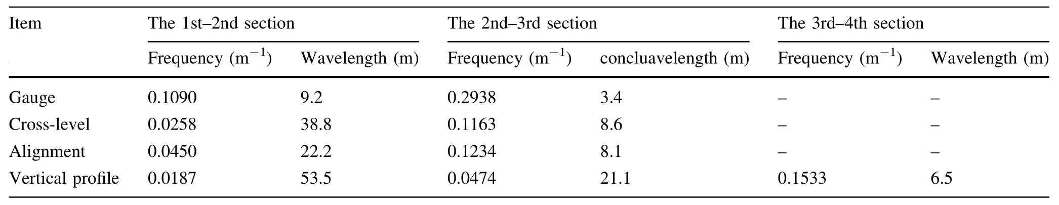
Table 2 The spatial frequency and corresponding wavelength of sectional points for the spectrum

·German high-speed low-disturbance spectrum [2]:

whereSv,SaandSxdenote the power spectral density of vertical profile irregularity,alignment irregularity and cross-level irregularity,respectively;Ω denotes the spatial wavenumber,in rad/m;truncated wavenumbers Ωc=0.8246 rad/m and Ωr=0.0206 rad/m;and for low-disturbance spectrum,coefficientsAv=4.032×10-7m·rad,Aa=2.119×10-7m·rad,andb=0.75 m.

Set the time-domain track irregularities transformed from above two track irregularity spectrums as system excitations,as shown in Fig.13.Figure 14 presents the comparisons of car body lateral and vertical accelerations under these two different excitation conditions,from which the car body accelerations excited by the China spectrum are far smaller than those by German spectrum,e.g.,the maximum car body lateral and vertical accelerations are,respectively,0.0025gand 0.0129gfor the China spectrum,and 0.0081gand 0.0383gfor German spectrum.Besides,the car body acceleration by China spectrum is smaller than that by German spectrum at almost all frequencies.

Figure 15 further presents the comparisons on wheel–rail forces.The maximum wheel–rail lateral and vertical forces are,respectively,8.68and136.63kN with respectto the China spectrum,and10.04and150.94kN for the Germanspectrum,namely the maximum wheel–rail forces excited by the China spectrum are also smaller than those excited by German spectrum.However,it is noted that the wheel–rail forces excited by the China spectrum are larger than those by the German spectrum at frequencies above 101.7 and 83.03 Hz.

Apart from the comparison on typical train dynamics,influence of track irregularities on track–substructural system responses can be evaluated.From the results,the maximum rail vertical acceleration subject to the excitation of China spectrum is 193.05 m/s2,but only 75.34 m/s2for German spectrum.The reason lies in the high sensitivity of the rail beam to high-frequency excitations.As displayed in Fig.15,German spectrum possesses better status in highfrequency track irregularities compared to the China spectrum,and consequently,the rail acceleration against China spectrum at the high-frequency domain is significantly larger than that of the German spectrum.

As to the track slab,tunnel segment and bridge girder accelerations,the maximum lateral and vertical accelerations are listed in Table 3.It can be seen from Table 3 that the vertical accelerations of the track slab,tunnel,andbridgewith respect to China high-speed spectrum are smaller than those with respect to German low-disturbance spectrum.It is found that the lateral accelerations of the track slab and tunnel under China spectrum excitations are obviously larger than those of the German spectrum.It can be observed from Fig.16thatthe differences of tunnel lateral acceleration shown in Fig.17 with respect to these two track spectrums mainly exist in frequencies larger than 101.7 Hz,where the tunnel lateral acceleration excited by China high-speed spectrum is significantly larger than that excited by the German low-disturbance spectrum,and it causes the larger values of tunnel lateral acceleration excited by China spectrum.

Table 3 Maximum track and substructural acceleration

5 Conclusions

An original method for solving large-scale train–track–substructure dynamic interaction has been presented in this paper for the first time.The numerical model is based on a coupled train–track model and substructural finite element models and solved in the time domain.In a robust and costeffective manner,substructures are modeled as independent matrices including their interaction matrices to the upper track.The train–track system is coupled as an entire one by matrix equations,only demanding a rather limited modeling length,namely satisfying being larger than the total length of a train and two times the boundary length,and then,the infinite length of a train moving on tracks can be achieved by a cyclic calculation method.An ingenious tactics is developed to consider the vibration participation of multiple substructures,such as tunnel and bridge,in the train–track interaction process at arbitrary time or position by DOF mapping relation and iterative solution.

Numerical applications show that this model is equally accurate to the train–track–substructure coupled solution,but with higher efficiency and less computer storage consumption.Numerical studies have shown that the substructures have relatively slight influence on train dynamic behaviors,e.g.,the car body vertical acceleration and wheel–rail vertical force are increased by 7% and 4.83%,respectively.However,the track structure vibrations are significantly influenced no matter on response amplitudes or on response frequencies,besides,the train–track system responses are generally amplified at the low-frequency domain,but the sensitive frequencies are different for different sub-systems,depending on the parametric properties of the substructures.Moreover,the influence of track irregularities on train–track–substructure system performance has also been clarified.It has proved that the high superiority of China high-speed spectrum in controlling middle–long wavelength irregularities but being worse in short-wavelength irregularities compared to the German low-disturbance spectrum.

AcknowledgmentsThis work was supported by the National Natural Science Foundation of China (Grant No.52008404),and the National Natural Science Foundation of Hunan Province (Grant No.2021JJ30850).

Open AccessThis article is licensed under a Creative Commons Attribution 4.0 International License,which permits use,sharing,adaptation,distribution and reproduction in any medium or format,as long as you give appropriate credit to the original author(s) and the source,provide a link to the Creative Commons licence,and indicate if changes were made.The images or other third party material in this article are included in the article’s Creative Commons licence,unless indicated otherwise in a credit line to the material.If material is not included in the article’s Creative Commons licence and your intended use is not permitted by statutory regulation or exceeds the permitted use,you will need to obtain permission directly from the copyright holder.To view a copy of this licence,visit http://creativecommons.org/licenses/by/4.0/.

Appendix

See Tables 4–7.

Table 4 Main parameters of the vehicle

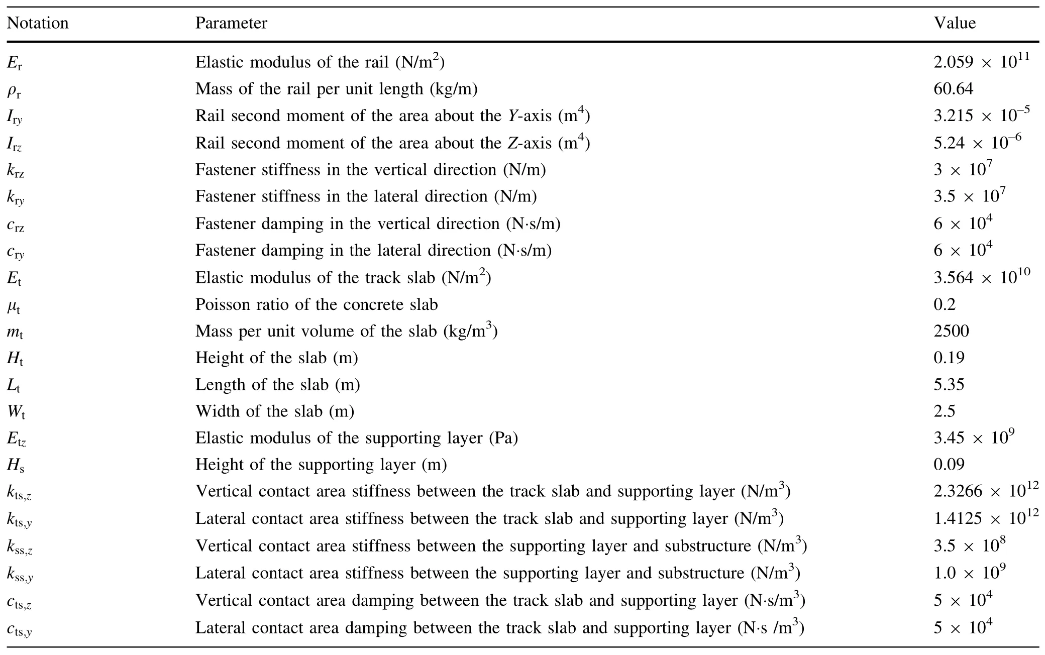
Table 5 Main parameters of track structures

Table 6 Main parameters of the tunnel

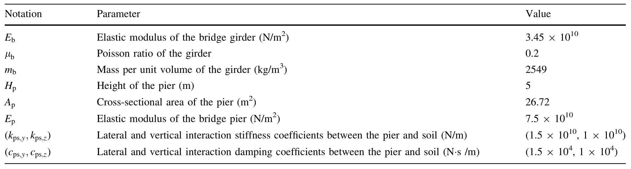
Table 7 Main parameters of the bridge girder and pier