Centrifuge modelling of ground-borne vibrations induced by railway traffic in underground tunnels

Yang Wenbo, Qian Zhihao, Tu Jiulin, Zhou Ziyang, Yan Qixiang, Fang Yong and He Chuan

Key Laboratory of Transportation Tunnel Engineering, the Ministry of Education, Southwest Jiaotong University, Chengdu 610031, China

Abstract: Increased attention has been given to ground-borne vibrations induced by railway vehicles and to the effects of these vibrations as they propagate through the ground into nearby buildings. Various studies, mainly based on numerical methods as well as physical modelling, have been carried out to investigate this problem. To study the dynamic response of tunnels and the surrounding soil due to train-induced vibration loads, a centrifuge test was conducted with a small-scale model in 1 g and 50 g stress field environments. An aluminum tube was embedded in sand to model the underground tunnel. A small parallel pre-stressed actuator (PPA) was employed to apply vibration loads on the tunnel invert. The model responses were measured using accelerometers. Both time and frequency domain analyzes were performed. The test results demonstrated that electronic noise had a clear impact on the test results and should be eliminated. It also found that the dynamic response of both the tunnel and soil were affected by the stress field. Therefore, it is important to account for the stress field effects when assessing the ground-borne vibration from tunnels.

Keywords: centrifuge test; stress field; frequency response function; peak particle acceleration; dynamic response

1 Introduction

Underground rail transit has gradually evolved into a complex transportation system. Meanwhile, the groundborne vibration induced by railway vehicles has become an increasing environmental concern that must also be considered. Vibrations from underground tunnels due to the dynamic interaction between the railcar wheel and rail can be transferred through the surrounding soil strata and into the nearby buildings which could significantly affect the comfort and safety of residents (Guptaet al., 2009; Croyet al., 2013). In addition, train-induced vibrations can cause other impacts on the tunnels, such as secondary deterioration caused by long-term vibration loads. It is of great significance, therefore, to understand the mechanism whereby train-induced vibrations propagate.

At present, various studies have been performed to investigate the dynamic response of tunnels and the surrounding soils under train-induced vibration loads, and some advancements have been made (Xiaet al., 2009; Zhaiet al., 2010; Huanget al., 2015; Sunet al., 2016; Baziaret al., 2016; Fuet al., 2016; Yanget al., 2020). One way to study ground-borne vibration induced by railway loads is through the use of physical modelling tests. Only a limited amount of research has been performed in this area. Tamuraet al. (1975) and Asano and Kumagai (1978) , whose work was discussed in Tsunoet al. (2005), are regarded as the pioneers in the field; they developed models to study vibrations from underground trains. Tamuraet al. (1975) conducted a test using a 1:100 scale model to study the deformation of a model tunnel due to an excitation force applied by a small shaker. Asano and Kumagai (1978) tested a 1:19.2 scale model of the Shinkansen tunnel to study the propagation of ground-borne vibration in the loam layer due to an impulsive load provided by a dropping ball system and a harmonic load provided by a vibration shaker. Trochides (1991) used a 1:10 scaled model excited by a shaker at normal gravity to measure the model response in the 500-5000 Hz frequency range. Thusyanthan and Madabhushi (2003) tested two tunnel models using different materials and studied how the lining materials affected the dynamic response of underground structures when subjected to surface loads. Based on frequency domain analysis, Yanget al. (2018) calculated the dynamic response of the tunnel and surrounding soil due to train-induced vibrations, including the influence of segment joints (Yanget al., 2017) and dome voids (Yanget al., 2019) on the response characteristics of the tunnel lining and surrounding soil.

Extensive research has been undertaken to determine the propagation of train-induced vibration in soil using numerical two-dimensional (2D) models (Krylov, 1995; Joneset al., 2002; Andersen and Jones, 2006; Aielloet al., 2008) and three-dimensional (3D) models (Wolf, 2003; Yaseriet al., 2014; Realet al., 2015), but these models have some disadvantages. The 2D models cannot account for wave propagation in the longitudinal direction of the tunnel, while the 3D models have low computational efficiency. One way to overcome the shortcomings of the conventional models is to build advanced models. As a result, a variety of 2.5D models in which the geometry of the system in the longitudinal direction is assumed to be invariant and the solution is required over only the cross section (Maet al., 2019) have been developed in recent years. These include the coupled finite element-infinite element model (Yanget al., 2003), the Pipe-in-Pipe model (Forest and Hunt, 2006; Hussein and Hunt, 2007; Husseinet al., 2014), the discrete wavenumber finite and boundary element methods (Shenget al., 2006), the coupled finite element method and method of fundamental solutions model (Amado-Mendeset al., 2015) and the coupled finite element and perfectly matched layer model (Lopeset al., 2014, 2016).

All of the above studies were conducted by using a physical modelling method in normal gravity (1 g) or a numerical simulation approach. The geotechnical centrifuge can more accurately reproduce the stress field of the prototype in the small-scale model. In such experiments, the dynamic shear modulus and damping ratio are two key parameters for studying the dynamic response of underground tunnels and the surrounding soil. However, the dynamic shear modulus and damping usually vary with depth due to the increase in confining stress in the actual stress field. The dynamic shear modulus of the soil layer used in the centrifuge was calculated using the empirical relationship proposed by Hardin and Richart (1963) for round grained sand at the strain levels ofγ=10-4based on laboratory tests. In addition, the relationship between the damping and confining stress has been studied by Assimakiet al. (2000) and Delfosse-Ribayet al. (2004). Seedet al. (1986) concluded that the magnitude of the sand damping ratio can be very high at very low-confining stress (less than about 25 kPa). Rollinset al. (1998) found that for gravelly soils the confining stress increased from 50 kPa to 400 kPa, while the damping values decreased at strain levels of 0.001%–1%.

This paper presents the results of a program of geotechnical centrifuge testing undertaken to study the influence of stress levels on ground-borne vibrations induced by underground railway traffic. The centrifuge modelling of ground-borne vibrations induced by underground railways are outlined in Section 2, and a reliability analysis of the measured results is given in Section 3. A comparison and discussion of the experimental results for the tunnel and soil at different stress fields are given in Section 4 and Section 5, respectively. The conclusions are presented in Section 6.

2 Centrifuge model test

Research in the dynamic behavior of tunnels, the surrounding soil and buildings under vibration loads have been conducted by many researchers, but most have focused on numerical simulations and physical modelling tests in a 1 g environment. However, it is well known that the soil behavior greatly depends on the initial stress state. To correctly model the dynamic behavior of the soil, this study used centrifuge modelling to understand the effects of ground-borne vibrations from tunnels.

2.1 Experimental model

The principle of centrifuge modelling is that by scaling the dimensions of a prototype by a factor ofN, whilst at the same time increasing the body force applied to the model by centrifugal acceleration at the same scale, the stresses in the model soil remain the same as those in the prototype. In this test, the TLJ-2 geotechnical centrifuge at Southwest Jiaotong University (SWJTU) was used to test the dynamic behavior of the tunnel and the response of the surrounding soil at different g levels. The geotechnical centrifuge is shown in Fig. 1. The centrifuge has an effective rotating radius of 2.70 m, the centrifugal acceleration range is 10–200 g, and the maximum payload capacity is 100 g∙t (g∙t refers to the product of unit of gravity acceleration and unit of weight).

Fig. 1 TLJ-2 geotechnical centrifuge of SWJTU

All the scaling factors were theoretically derived, based on the results given in Iaiet al. (2005) in terms of the fundamental scaling factors for length (λ), density (λρ), strain (λε), and acceleration of gravity or centrifugal acceleration (λg). The scaling factors for the centrifuge model tests are shown in Table 1; the acceleration was scaled byλg= 1/λconsistent with the geometrical scaling factorλand the soil material had the same density as the prototype and model (i.e.,λρ=λε= 1).

To simulate the three-dimensional propagation of ground vibration, a steel container with a length of 0.8 m, width of 0.6 m and height of 0.6 m was used (Fig. 2). The reflection of vibration waves on the rigid boundary of the container was one of the main problems encountered in the test. To minimize this effect, a 25 mm thick layer of vibration absorbing material, Duxseal, was attached to the inner wall of the container to absorb the incident waves at the boundaries (Pak and Guzina, 1995; Yanget al., 2013, 2020).

Fig. 2 Model container and tunnel

Quartz sand, supplied by the Key Laboratory of Transportation Tunnel Engineering of the Ministry of Education at Southwest Jiaotong University, was selected as the soil material for the experiments. To achieve a uniform distribution of the soil, the sand was placed in a hopper and sifted through a slotted plate from a constant height (Yanget al., 2013). The relative density and the density of the model soil were determined to be 63% and 1610 kg/m3. The properties of the sand are given in Table 2. A cylindrical aluminum tube with an inner diameter of 108 mm and a thickness of 6 mm was embedded in the sand to model the underground tunnel. The properties of the tunnel are shown in Table 2 and the geometric parameters are given in Table 3.

Table 1 Scaling factors for centrifuge test

Table 2 Properties of tunnel and sand for centrifuge test

The two ends of the tunnel were sealed to prevent sand ingress and the overlying soil was 330 mm thick. The inner diameter of the prototype tunnel was 5.4 m, the lining thickness was 0.3 m and the tunnel was buried at 16.5 m. During the centrifuge test, the centrifuge model was rotated at a speed of 129 rpm, with a corresponding angular velocity of 13.47 rad/s, and a centrifugal acceleration of 50 g at a radius of 2.70 m. To ensure that the test model reached a stable state, the machine was run for 20 minutes before the centrifuge test was conducted and the excitation signal was applied.

2.2 Experimental scheme

The alternating current used in the centrifuge produced strong current interference, and the output signal was therefore affected when it passed through the signal channel of the centrifuge. Therefore, the authors prepared two experimental schemes to allow a comparative analysis. The main test equipment in the test included: the TLJ-2 centrifuge, the signal generator (JM-1230), the signal amplifier (V-LA75C), the Parallel Pre-stressed Actuator (PPA20M), the dynamic force sensor (JM0710-001), the acceleration sensors, and the data acquisition equipment. The devices are shown in Fig. 3. The size and mass of some instruments are given in Table 4. The specific schemes are as follows:

Table 3 Geometric parameters of the tunnel

Table 4 Instrument size and mass

Scheme One (T1): As shown in Fig. 3, all the test equipment was located in the operating room; Computer I transfers the vibration signal to the signal generator (JM-1230), which then transmits the converted electric signal to the power amplifier (V-LA75C). The converted electric signal is then sent to the Parallel Pre-stressed Actuator (PPA20M) that is vertically installed at the bottom of the tunnel allowing a vertical excitation load to be applied to the tunnel. The force sensor (JM0710-001) in conjunction with the Parallel Pre-stressed Actuator was employed to measure the vibration force. To analyze the dynamic behavior of both the tunnel and the soil due to the vibration load, 15 acceleration sensors were arranged at different positions in the tunnel and at different depths in the soil above the tunnel. The arrangement of the accelerometers is shown in Fig. 4. All the accelerometers were used to measure the vertical accelerations. Four accelerometers were arranged at the tunnel invert (A1, A2, A3, A4), and three accelerometers were bottled at the vault (A5, A6, A7) to record the tunnel response. Six accelerometers were placed within the interior of the soil, and two accelerometers were placed at the soil surface to record the soil response. All the sensor cable joints were connected to the centrifuge, and the response measured by the sensors was transmitted through the signal channel of the centrifuge to the data acquisition instrument in the operating room. The data acquisition instrument converted the dynamic response captured by the sensors into a digital signal, which was then transmitted to the computer.

Fig. 3 Test instruments

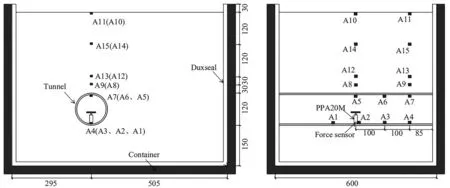
Fig. 4 Location of the accelerometers (all dimensions in mm)

Scheme Two (T2): Computer I (Fig. 3) and Computer Ⅱ (Fig. 1) were connected via a wireless local area network (LAN) before the data acquisition device and Computer Ⅱ were fixed to the centrifuge.Computer I in the control room remotely controlled the Computer Ⅱ to send a signal; the electrical signal converted by the signal generator was transmitted to the power amplifier and then to the Parallel Pre-stressed Actuator after amplification. With this driving signal, the actuator applied a dynamic force to the model. After the model was excited, the dynamic responses captured by the sensors were transmitted to the data acquisition equipment, and the converted digital signal was recorded in Computer Ⅱ. The measured data was streamed to the hard disk, and further analysis was performed in MATLAB. The output signal did not pass through the signal channel of the centrifuge when the response was recorded, effectively eliminating any interference from the alternating current of the centrifuge. The positioning of the accelerometers in this scheme (T2) was the same as that of Scheme One (T1).

The loads shown in Fig. 5 are the prototype loads which are calculated according to the similarity ratio in Table 1. The vibration loads applied to the tunnel were sweep loads and train-induced vibration loads. According to the Nyquist-Shannon sampling theorem, the sampling frequency should be at least twice the maximum frequency component of the measured signal. Therefore, the sampling frequency in the experiment was 64000 Hz, which is sufficient to represent the accuracy of the signal waveform.

(1) Sweep load. According to Yanget al. (2018), the frequency response function (FRF) curve is not affected by the sweep signal itself (such as the sweep amplitude, the sweep direction, and the sweep period). To study the dynamic response of the tunnel structure and the surrounding soil at different frequencies, a sinusoidal sweep load with a frequency of 0–10000 Hz (the corresponding frequency range in the prototype is 0–200 Hz) was applied on the model tunnel, with a sweep period of 15 s and a sweep amplitude of 300 mv. The sweep excitation force curve is shown in Fig. 5(a).

Fig. 5 Curves of excitation load for (a) sweep-frequency excitation load, (b) train-induced load at 40 km/h, (c) train-induced load at 50 km/h, and (d) train-induced load at 60 km/h

(2) The train-induced load. In the centrifuge experiment, a train-induced load was applied at different speeds (40 km/h, 50 km/h, 60 km/h). Furthermore, the influence of the train speeds on the peak particle acceleration at each measurement point in the tunnel lining and within the interior of the soil under different stress fields was analyzed. The load curves are shown in Figs. 5(b)–5(d).

3 Frequency response function and the reliability analysis of the measured results

3.1 Frequency response function and the coherence function

To compare the test results, the results of the centrifuge test at 50 g were scaled to the idealized prototype at 1 g. Typical time histories of the tunnel and soil response are shown in Fig. 6. The time domain results were converted into frequency domain results, and the frequency response functions (FRFs) of the model were calculated. The frequency response function is defined as the ratio of the Fourier transform acceleration response to the vibration load. To reduce the influence of noise on the data and reduce random error, the measured time domain data were regarded as random samples, and the dynamic responses of each measurement point were analyzed by random vibration theory. The frequency response functions are calculated by Eq. (1):

Fig. 6 Typical time histories of the model response due to sweep-frequency load taken at two locations in the tunnel ((a), (b)) and two locations in the soil above the tunnel ((c), (d))

The coherence function provides a quantification of the correlation between the response signal and the force signal that is then introduced to examine the reliability of the measured results. The coherence function is defined as

The range of the coherence value is between 0 and 1. A coherence value of 0 indicates that the response of the observation points has nothing to do with the vibration excitation. A coherence value of 1 indicates that the dynamic response is completely induced by the excitation; thus, the quality of the measured results is reliable. The coherence function is calculated using Eqs. (3)–(6):

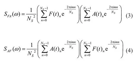
wherem= 1, 2, …,NS– 1;n= 0, 1, 2, …,NS– 1;ωis the frequency,F(t)nis the measured excitation force,A(t)nis the measured responses,SFA(ω) is the cross-spectrum of the force and response,SAF(ω) is the cross-spectrum of response and force,SFF(ω) is the auto-spectrum of force, andSAA(ω) is the auto-spectrum of response (Yanget al., 2013).

3.2 Effect of current noise on the frequency response function

In the experiment, two experimental schemes were used for comparative analysis to prove that the alternating current of the centrifuge will impact the test results. A comparison of the results from schemes T1 and T2 for the tunnel and soil response at 1 g and 50 g are shown in Figs. 7 and 8, respectively.

The following characteristics can be deduced from the Fig. 7: the test results of T1 and T2 have a good consistency because there is no interference from the centrifuge alternating current at 1 g. Specifically, the model shows the same behavior in the two tests except in the low-frequency range. The reason for this is that the measured data in the low-frequency range is sensitive to interference from external environmental noise. In addition, there is a slight difference (less than 4 dB) over the high-frequency range for the FRFs plot. This can be explained by the inherent uncertainties in the model test preparation, such as slight deviations in the position of the model tunnel and the accelerometers.

At 50 g, the two model responses exhibit similar trends, as shown in Fig. 8. However, the results of the response for the tunnel and soil from the two tests were not as good as the results in Fig. 7; the FRF curves of the T2 scheme were obviously smoother than the results for the T1 scheme. These differences are due to the unavoidable strong current disturbances in the T1 scheme, proving that the current noise has a significant impact on the test results, with better test results obtained for the T2 scheme, which greatly reduced the problems associated with the data processing.

Fig. 7 FRF curves of the model tests at 1 g: (a) point A2 on the interior tunnel wall, (b) A10 on the soil surface

Fig. 8 FRF curves of the model tests at 50 g: (a) point A2 on the interior tunnel wall, (b) point A10 on the soil surface

3.3 Reliability analysis of the measurement results

The FRF curves at the measurement points A3 and A5 (tunnel), A14 and A10 (soil) and the corresponding coherence functions for the whole frequency range are shown in Fig. 9 (in which the red curve represents the coherence curve of the measurement points, and the black curve represents the frequency response functions (FRFs)).

It was found that the FRF curves and coherence values in the full frequency ranges show different variational patterns (Fig. 9). The FRF curves and corresponding coherences in the frequency range 0–10 Hz fluctuate dramatically, mainly because the measured data in the low-frequency range is susceptible to interference from external environmental noise generated by the centrifuge drive system. When the excitation frequency was within the range 10–40 Hz, the coherence increased gradually, which indicated that the effect of noise on the measured tunnel and soil responses was weakened gradually, and the responses were gradually controlled by the vibration excitation. When the frequency was greater than 40 Hz, the coherence function values were all close to 1. Although there were troughs in some frequencies, the overall trend was better in the frequency range, which indicates that the response of the tunnel and soil were well correlated and the measured response was 100% due to the excitation force; thus, the test results are relatively reliable.

Fig. 9 FRF curves and corresponding coherence function for tunnel measurement points (a) A3 and (b) A5, and soil measurement points (c) A14 and (d) A10

Note that the measured tunnel response was better than the measured soil response because the excitation was applied within the tunnel and any external noise had less of an effect on the tunnel response. In addition, the data from within the soil was better than that recorded at the surface, which is because the effect of noise is proportionately higher because the magnitude of the measured signal within the soil was greater than the signal magnitude at the surface. Based on the above analysis, the current work mainly focused on the dynamic behaviors of the model within the frequency range of 40–200 Hz.

4 Dynamic behavior of the tunnel

4.1 Dynamic response of the tunnel - time domain results

Vibration from underground tunnels is generated by the dynamic interaction between the wheel and rail caused by irregularities in the wheels and tracks. These vibrations can be transferred through strata overlying the tunnel and into nearby buildings. In the experiment, three different train-induced vibration loads caused by different speeds were applied to the invert of the tunnel. A comparison between the data measured in the 1 g environment and in a 50 g environment at peak particle accelerations of each measurement point in the tunnel is given in Table 5.

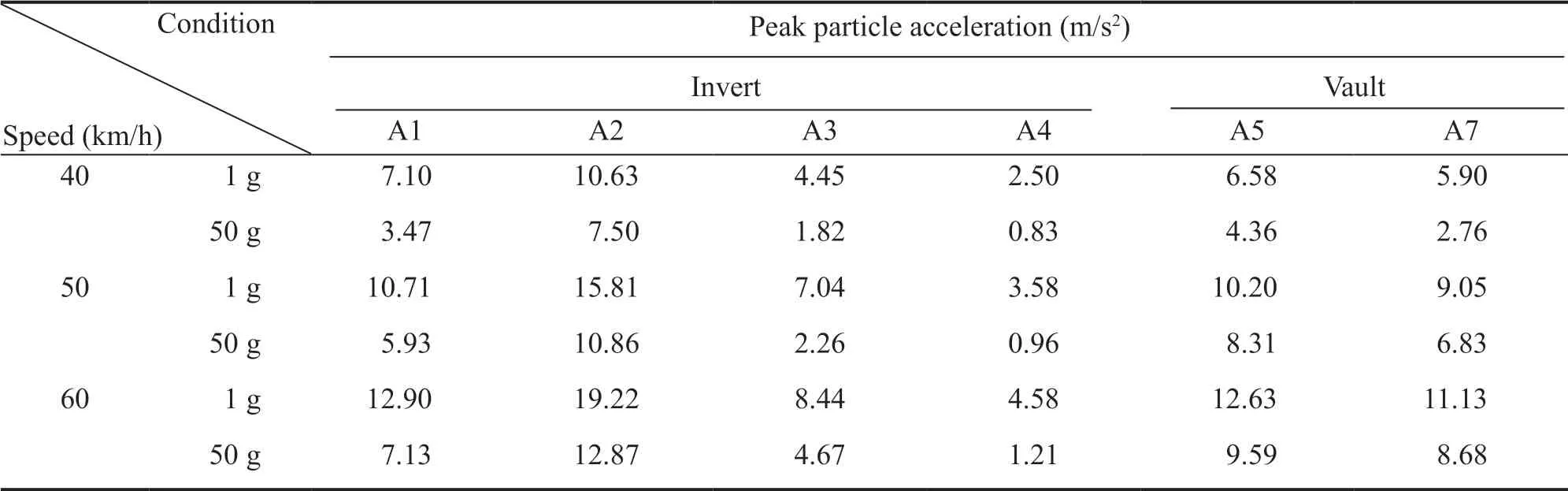
Table 5 Peak particle acceleration on the tunnel

The peak particle acceleration in the tunnel increases with an increase in the vehicle speed; however, the peak particle accelerations exhibit different degrees of attenuation at the invert and vault of the tunnel. The peak particle accelerations at the measurement points in the tunnel invert quickly decayed along the center line of the tunnel, while the degree of attenuation at the vault was very weak; this should be intensively monitored at the tunnel vault during the operation.

It was also found that the peak particle accelerations at the same points were also different at different stress fields; the peak particle acceleration of the model tunnel at 1 g was larger than that at 50 g. These differences were observed for the three different load speeds, 40 km/h, 50 km/h and 60 km/h. For instance, the peak particle acceleration for the observation point A5 in the 50 g environment was 9.59 m/s2due to the train-induced load with a speed of 60 km/h, while the value recorded in the 1 g environment was 12.63 m/s2, which was 1.32 times as much as that in the 50 g stress filed. This shows that the stress field had an influence on the dynamic response of the tunnel; the geometric damping and material damping of the tunnel varied because of the high stress field.

4.2 Dynamic response of the tunnel - frequency domain results

It has been difficult to study the dynamic behavior and attenuation of the tunnel and surrounding soil in response to vibration excitation. To analyze the threedimensional propagation of ground-borne vibration, the measured time domain results were converted into frequency domain results, and the FRFs of the model response were calculated. Some environmental noise disturbance was inevitable in the test. According to the analysis described in Section 3, the dynamic response of both the tunnel and the surrounding soil in the range of 40–200 Hz were specifically analyzed at different g levels. The FRF curves from the observation points at the invert and vault of the tunnel under 1 g and 50 g stress fields are shown in Figs. 10 and 11.

The response at a stress field of 50 g was greater than that in the 1 g environment, with a difference of about 20 dB. This indicates that the stress field has a great significant on the dynamic response of the tunnel. Within the frequency range of 40–100 Hz, the response increases slowly with an increase in frequency and gradually flattens. Though the frequency increases continually when it was greater than 100 Hz, the response remains in a stable range, which means that the increase in frequency may not lead to an increase in the tunnel response at this frequency range. In the longitudinal direction of the tunnel, the points were farther from the vibration source, and the corresponding responses were smaller; in other words, the responses exhibited a continually diminishing trend along the tunnel centerline. In addition, the measurement from the tunnel invert in Fig. 10(a) showed a higher response level than the measurement of the vault in Fig. 11(a). This could be because the existence of geometric decay and material damping leads to energy loss during the vibration propagation process along the depth and distance from the source.

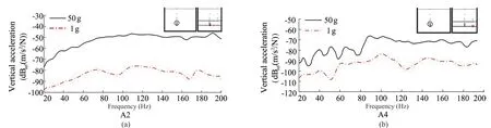
Fig. 10 FRF curves for (a) point A2 at the tunnel invert, and (b) point A4 at the tunnel invert

Fig. 11 FRF curves for (a) point A5 at the tunnel vault, and (b) point A7 at the tunnel vault

5 Dynamic behavior of the surrounding soil

5.1 Dynamic response of the surrounding soil - time domain results

The experiment also recorded the response from each observation point placed in the soil above the tunnel due to a train-induced load at different speeds; the peak particle accelerations were then extracted. The results are given in Table 6. By comparing the results from the three speeds (40 km/h, 50 km/h, and 60 km/h), it was observed that the peak particle acceleration at different depths in the soil increased with an increase in the vehicle speed. A similar phenomenon was also seen for the model tunnel. Moreover, it should be noted that the peak particle accelerations of the soil at a stress field of 50 g were significantly greater than those recorded in the 1 g environment. For instance, the peak particle acceleration of the surface observation point A10 at a stress field of 50 g was 5.97 times as much as for the stress field of 1 g under a train-induced load at a speed of 60 km/h. The reason for this phenomenon is that the damping value of the soil reduces and the stiffness of the soil increases at the high-stress level, so that the peak particle acceleration at the measurement points within the interior of the soil was greater under the 50 g condition.

Table 6 Peak particle acceleration in the soil

It was also observed that the dynamic response of the soil had an amplification effect on the surface of soil. The peak particle acceleration at the measurement points on the soil surface was greater than the peak particle acceleration measured at other locations within the interior of the soil. Yanet al. (2006) conducted field measurements on urban subways and showed that the propagation of vibration was amplified at the ground surface. This was consistent with the phenomenon observed in the experimental results and further verified the reliability of the results.

5.2 Dynamic response of the surrounding soil - frequency domain results

To analyze the dynamic response characteristics and attenuation law in the upper soil layer of the tunnel, eight accelerometers were arranged within the soil. The FRF curves of the soil response are shown in Fig. 12. The following two characteristics can be found through the analysis.

Fig. 12 FRF curves for (a) point A8, and (b) point A12

The dynamic response in the soil at a stress field of 50 g was significantly larger that at 1 g, which was consistent with the results observed in the tunnel structure, although the difference in the response at different g levels was greater than that observed in the tunnel. When the frequency was within the range of 40–100 Hz, the soil response increased slowly with the increase of frequency, and the difference in the dynamic response at different stress fields was relatively stable. However, the dynamic response decreased with an increase in frequency when the frequency was greater than 100 Hz. In the near field, i.e., A8, located close to the tunnel, the difference in response increased sharply for the two different stress fields, indicating that, at high frequencies, the soil response in the near field could be significantly affected by the stress field.

The reason for the above observations was that the damping of soil material varied under the high stress level, and the soil damping decreased due to the high confining pressure. A similar conclusion was described in Rollinset al. (1998), indicating that the stress field had an obvious influence on the dynamic response of the soil around the tunnel structure, and this influence should be fully considered.

6 Conclusions

An experimental study of the ground-borne vibration from an underground tunnel was conducted utilizing a centrifuge test. The study aimed to provide insight into the effect of the stress field on the three-dimensional propagation of ground-borne vibration from tunnels. The effects of the stress field on the dynamic behavior of the tunnel and surrounding soil were studied using the peak particle acceleration and frequency response function as an evaluation index. According to the results obtained from the centrifuge test for modelling vibration, the following conclusions can be drawn:

● The centrifuge test was successful in studying the ground-borne vibration induced from an underground tunnel. Due to the significant effect that electrical noise had on the measured data, a scheme was devised that effectively improved the results.

● The experimental results showed that the stress field had a significant effect on the model response when the dominant frequencies of the tunnel and surrounding soil induced by railway traffic were above 40 Hz. The response of the tunnel and soil due to a sweep load at a 50 g stress field was greater than that at a 1 g stress field, and the average difference in the tunnel response was less than 20 dB. However, the difference in the soil was more significant in the near field, and could reach up to 30 dB at high frequencies. The reason was that the increase in the confining pressure reduced the damping of soil; thus, the model response at a 50 g stress field was greater.

● The results of the peak particle acceleration were compared to the results for the effect of vehicle speed on the tunnel and soil dynamic behavior. The comparison suggests that the peak particle acceleration increases with the increase in vehicle speed. The peak particle acceleration of the measurement points on the tunnel in the stress field of 1 g was 1.32 times as much as that in the 50 g environment, while the peak particle acceleration on the soil surface in the stress field of 50 g was 5.97 times as much as that in the 1 g environment. This further indicates that the influence of the stress field should be considered to effectively study the groundborne vibration from an underground railway.

In this study, the operational velocity of the train was either 40 km/h, 50 km/h or 60 km/h. There are much faster high-speed railways all over the world, for instance, the largest high-speed railway network, located in China, is the Fuxing Hao maximum network, with a current operational velocity of 350 km/h that is expected to reach 400 km/h in the near future. In addition, the maglev train′s operational velocity has reached 430 km/h. Therefore, the dynamic behavior of the tunnel and surrounding soils due to vibration loads from underground railway traffic at higher speeds than in this research should be investigated further.

Acknowledgement

This work was supported by the National Natural Science Foundation of China (No. 51678499).