Large deformation analysis of slope failure using material point method with cross-correlated random fields*

Chuan-xiang QU, Gang WANG, Ke-wei FENG, Zhen-dong XIA

Large deformation analysis of slope failure using material point method with cross-correlated random fields*

Chuan-xiang QU, Gang WANG†‡, Ke-wei FENG, Zhen-dong XIA

†E-mail: gwang@ust.hk

Large deformation analysis of slope failure is important for hazard and risk assessment of infrastructure. Recent studies have revealed that spatial variability of soil properties can significantly affect the probability of slope failure. However, due to limitations of traditional numerical tools, the influence of spatial variability of soil properties on the post-failure behavior of slopes has not been fully understood. Therefore, in this study, we aimed to investigate the effects of the cross-correlation between cohesion and the friction angle on the probability of slope failure and post-failure behavior (e.g. run-out distance, influence distance, and influence zone) using a random material point method (RMPM). The study showed that mesh size, strength reduction shape factor parameter, and residual strength all play critical roles in the calculated post-failure behavior of a slope. Based on stochastic Monte Carlo simulation, the effects of cross-correlation between cohesion and the friction angle on the probability of slope failure, and its run-out distance, influence distance, influence zone, and sliding volume were studied. The study also showed that material point method (MPM) has great advantages compared with the finite element method (FEM) in handling large deformations.

Material point method (MPM); Spatial variability; Random field; Large deformation; Risk assessment

1 Introduction

Slope failure can cause tremendous damage to infrastructure and threaten the lives of people. For example, a large-scale construction solid waste (CSW) landslide that occurred in Shenzhen in December 2015 resulted in 77 deaths and 33 houses destroyed (Yin et al., 2016). The occurrence of slope failure is affected by many uncertain factors, including external loads and the inherent spatial variability of soil properties. Wang MY et al. (2020) showed that ignoring the spatial variability of soil properties can lead to overestimation of the calculated factor of safety (FOS) of a slope. To evaluate potential slope failure risk appropriately, numerical approaches (e.g. random limit equilibrium method (RLEM) and random finite element/difference method (RFEM/ RFDM)) have been increasingly applied in reliability analysis of slope stability. For instance, Cho (2010) investigated slope stability by RLEM based on a Monte Carlo simulation (MCS) framework. Cheng et al. (2018) assessed potential slope failure risk using RFDM. Moreover, as simulating a small probability of slope failure (e.g.f<10−3) is particularly time-consuming, Li et al. (2016) and Wang MX et al. (2020) combined subset simulation (SS) with RFEM to improve computational efficiency.

However, slope failure is usually accompanied by a large run-out distance, influence zone, and sliding volume (Wang et al., 2018; Huang et al., 2020; Liu et al., 2020; Feng et al., 2021b). Classical limit equilibrium method (LEM), finite element method (FEM), and finite difference method (FDM) cannot model large deformation of slope failure and therefore can underestimate the risk of slope failure. Fortunately, the development and application of the material point method (MPM) can effectively deal with these limitations. MPM, as a hybrid Eulerian-Lagrangian method, combines the advantages of both schemes (Sulsky et al., 1994, 1995). It can avoid mesh distortion by using a fixed Eulerian background grid for interpolation, and becomes suitable for simulating large deformation problems. MPM has been increasingly applied to simulate the dynamic process of slope failure. For example, Bandara and Soga (2015) and Soga et al. (2016) coupled soil deformation and pore fluid based on MPM, and then simulated progressive failure of river levees. Wang et al. (2016b) modeled two kinds of slope failure modes (progressive and retrogressive) by MPM. The use of MPM for the simulation of rainfall-induced slope failure has also been reported (Yerro et al., 2015; Bandara et al., 2016; Wang et al., 2018; Liu et al., 2020; Feng et al., 2021a).

Although MPM has been proven to be an effective and accurate numerical tool when studying large deformation problems, few applications of MPM have considered the inherent spatial variability of soil properties. Wang et al. (2016a) first proposed a random material point method (RMPM) to model a clay slope failure. Liu et al. (2019) further integrated RLEM and RMPM to simulate four types of slope failure modes. However, they considered variation of only a single parameter (i.e. the undrained shear strength of clays) and did not extend their results to more general soils. Previous studies showed the cross-correlation coefficient (ρ,ϕ) of cohesionand the friction anglecould significantly affect slope stability (Cho, 2010; Li et al., 2015; Liu et al., 2017; Wang MX et al., 2020; Ng et al., 2021). Nevertheless, most studies focused mainly on the triggering of slope failure (i.e.f), due to the limitations of numerical tools. The effects ofρ,ϕon the post-failure features of slopes, including the run-out distance, influence distance, and influence zone, have not been fully investigated.

To solve these problems, RMPM was selected to further investigate large deformations of slope failure in spatially variable soils. The main objective was to investigate the effects ofρ,ϕon the post-failure behavior of slopes. In Section 2, the computational procedure of RMPM is introduced. The cross-correlated–random fields are generated by the Cholesky decomposition technique. In Section 3, we discuss the impacts of influencing factors (i.e. mesh size, strength reduction shape factor parameter (), and residual strength) using homogenous slope profiles. In Section 4, the post-failure consequences of slopes with spatially variable soil properties are calculated by RMPM based on an MCS framework, in terms of the run-out distance, influence distance, influence zone, and sliding volume. Finally, the slope failure probability,f, and corresponding failure consequences are used to evaluate the potential risk of slope failure.

2 Random material point method

2.1 Material point method

MPM can be considered as an FEM variant used to simulate large deformation problems in geotechnics, and consists of a Eulerian background grid and Lagrangian material points. In this study, it was applied to investigate slope failure under gravity, hence, a total-stress, single-phase MPM was used. The calculation steps of MPM are summarized in Fig. 1: (a) mapping the information of material points (e.g. mass, velocity, and volume) onto the computational grid; (b) calculating the equilibrium equations on the grid; (c) interpolating updated nodal velocity and acceleration back to the material points, and then updating stress and history variables by a continuum constitutive model; (d) updating the particle positions, and starting a new iteration step.

The momentum balance equation and stress-strain relationship for a single-phase continuum are shown as

whereis the density;is the acceleration;is the unit body force;anddenote the total stress and strain, respectively;represents the tangent modulus defined by a constitutive model. In this study, the strain-softening Mohr-Coulomb constitutive model (Abbo and Sloan, 1995) was selected to describe the soil response:

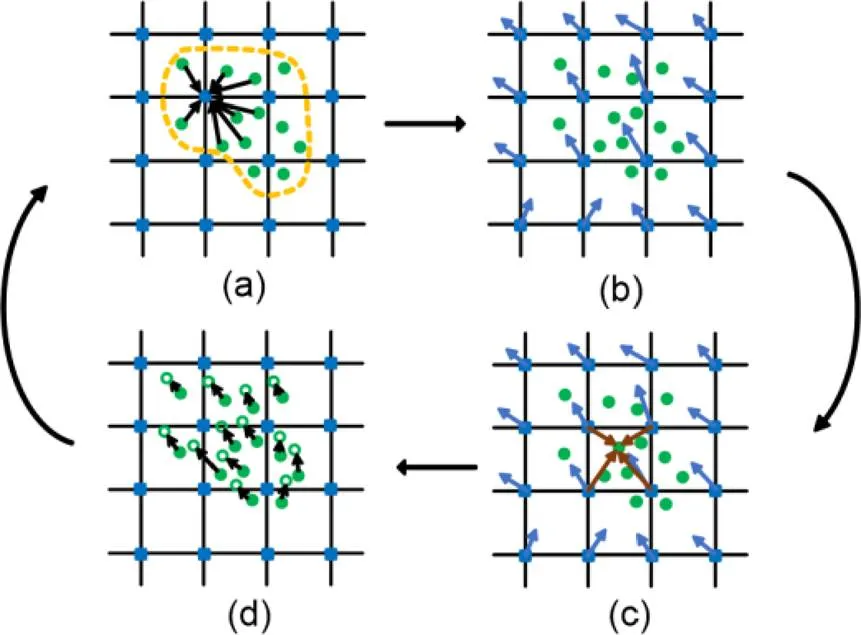
Fig. 1 A simulation cycle of MPM

(a) Particle to node; (b) Nodal computation; (c) Node to particle; (d) Update particles

2.2 Generation of cross-correlated c–ϕ random fields

Random field theory (Vanmarcke, 1983) has been popularly used in characterizing the spatial variability of soil properties. Here, cross-correlated non-Gaussian–random fields were adopted. Following Zhu and Zhang (2013), an exponential autocorrelation function (ACF) was adopted to simulate the spatial correlation of each soil property (or), as follows:

Once the ACF is determined, the autocorrelation matrix,(e×e) for a random field containingenumber of elements can be constructed:

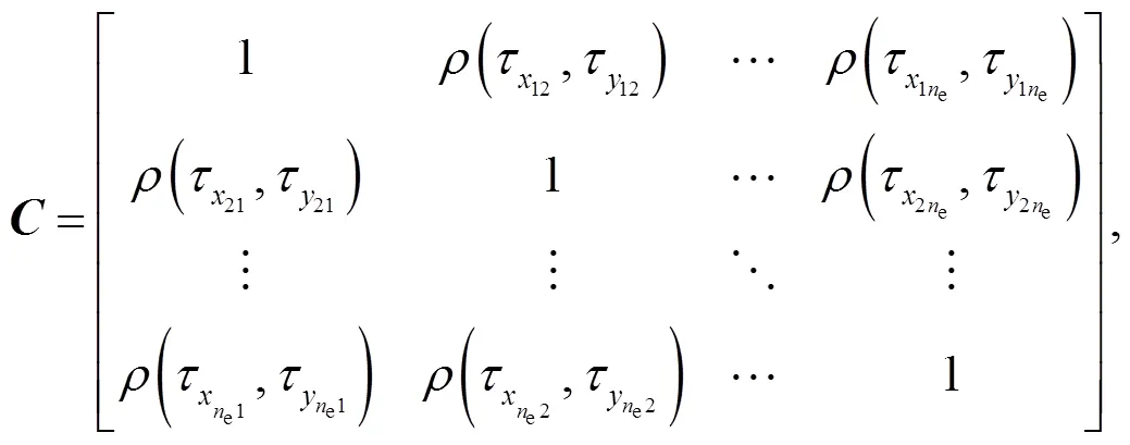
where both1(e×e) and2(2×2) are the lower triangular matrices. Finally, the cross-correlated non-Gaussian random fieldsCNG(e×2) can be generated by

2.3 Computational process of RMPM

The aforementioned parts introduce the principles of MPM and random field generation. In this study, the generation of cross-correlated random fields was programmed using Matlab, and imported into the MPM program written in C++ language. The numerical model was simulated by a computer with an Intel i7-6700HQ CPU @ 2.60 GHz and 8 GB RAM. Fig. 2 illustrates the computation process of RMPM. Each step can be summarized as follows:

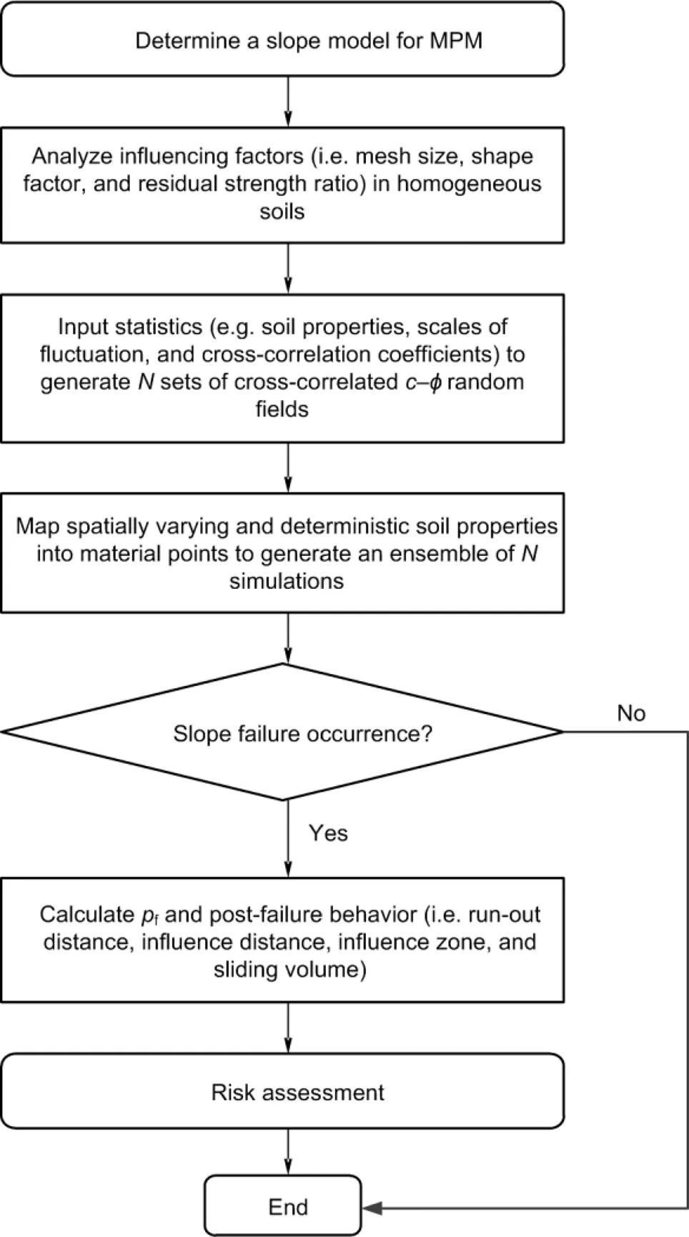
Fig. 2 Flowchart of RMPM calculation

1. Construct a slope model and determine the soil parameters. The strain-softening Mohr-Coulomb constitutive model was selected to represent the soil behavior.

2. Use a uniform soil profile to study the effects of influencing factors (i.e. mesh size, strength reduction shape factor, and residual strength ratio) on simulated results. Then, the analyzed results serve as references for stochastic analysis (Section 4).

3. Apply given statistics (e.g. mean values, coefficients of variation (COVs), cross-correlation coefficients, and scales of fluctuation) to generatesets of cross-correlated–random fields.

4. Assign deterministic and spatially variable soil properties to corresponding material points to generate an ensemble ofmodels.

5. Conduct MPM simulation for each realization. Here, a threshold displacement (0.4 m) was used to determine whether slope failure occurred (Wang et al., 2019). The slope failure probability is calculated byf=f/, wherefandrepresent the numbers of failure samples and total realizations, respectively.

3 Deterministic analysis of influencing factors

The strain-softening Mohr-Coulomb model can suffer from a mesh dependence problem, so a proper mesh size should be chosen to ensure accuracy of the simulation (Oliver and Huespe, 2004; Soga et al., 2016).The strength reduction shape factor parameter,, and the residual strength may also influence the simulated post-failure behavior of the slope. Thus, in this section, these influencing factors are investigated, and the results serve as references for the probabilistic analysis in Section 4. In this section, a homogenous soil profile (Fig. 3), was used to investigate these influencing factors. The height of the slope was 15 m with an inclination angle of 45°. The soil properties were shown in Table 1.

Fig. 3 Geometry of a homogenous slope

Table 1 Soil properties for a homogeneous slope

: unit weight;: Young’s modulus;: Poisson’s ratio

3.1 Effects of mesh size

In this part, the impacts of the mesh size on slope stability and failure consequences are analyzed. Using the soil parameters (peak strength) in Table 1, the FOS of the slope is 0.775 based on LEM, indicating that the slope is not statically stable. By changing the mesh size, a sensitivity analysis of FOS was conducted, and the post-failure behavior of the slope was investigated. The FOS was calculated by increasing the strength reduction factors of the peak strength parameters (pandp) without considering softening.

Each element in the mesh contained four material points. Four different mesh sizes, 0.25 m×0.25 m, 0.5 m×0.5 m, 1 m×1 m, and 2 m×2 m, were used, which correspond to 57 180, 14 310, 3585, and 900 material points, respectively. Fig. 4 shows the results from simulations under different mesh sizes. It is clear that the shear band becomes narrower and smoother as the mesh size decreases, as the thickness of a shear band is closely related to the mesh size in MPM calculation (Yerro Colom, 2015; Soga et al., 2016). The calculated FOS decreases as the mesh size decreases (Fig. 5). When the mesh size reduced from 0.5 m to 0.25 m, the calculated FOS was 0.772 and 0.758, respectively, which is close to the FOS calculated by LEM (0.775). On the other hand, with a decrease in the mesh size, the computational cost (CPU time) increases significantly. Therefore, selecting a proper mesh size is important in terms of the accuracy and efficiency of MPM calculation. Using a mesh size of 0.5 m seems to result in a similarly accurate result, while being more efficient than using a mesh size of 0.25 m.

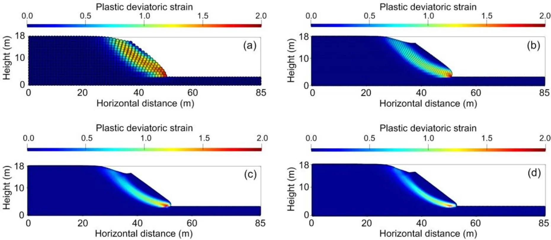
Fig. 4 Computed slope failure using different mesh sizes

(a) 2 m×2 m; (b) 1 m×1 m; (c) 0.5 m×0.5 m; (d) 0.25 m×0.25 m

Fig. 6 illustrates the quantitative measures of slope failure. The sliding depth was defined as the depth from the top of the slope to the lowest point in the sliding point. The sliding volume was calculated as the total volume of sliding material points. The run-out distance was calculated from the slope toe before failure to the forefront of the landslide. The influence distance was defined as the distance between the slope crest point before failure to the landslide crown after failure. Finally, the influence zone was measured as the sum of the influence distance, run-out distance, and the horizontal slope width.

Fig. 7 shows the calculated post-failure features of the slope under different mesh sizes. Reducing the mesh size could result in larger post-failure features (run-out distance, influence distance, influence zone, and sliding volume). All the results tended to converge when the mesh size was 0.5 m or 0.25 m, but the corresponding CPU times were 26.8 min and 119.2 min, respectively. Considering the significant saving of CPU time, we used a mesh size of 0.5 m throughout the study. The chosen mesh size can generate reasonably accurate results while enabling us to conduct a large number of MCSs, as higher computational efficiency is a key consideration. Therefore, the 0.5 m mesh size was used in the following analysis considering both the computational efficiency and accuracy. Note that Yerro Colom (2015) proposed a method such that, with a properly selected softening parameter, a coarser mesh can be used to gain results consistent with those from a finer mesh.

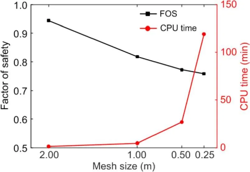
Fig. 5 Factor of safety and corresponding CPU time under different mesh sizes

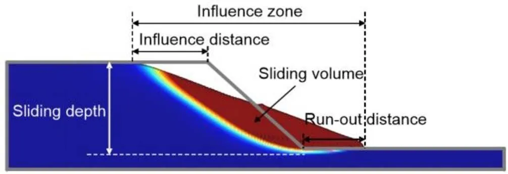
Fig. 6 Quantitative consequences of slope failure

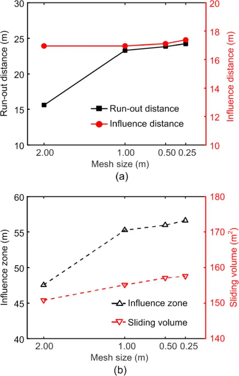
Fig. 7 Quantitative post-failure slope features under different mesh sizes: (a) run-out distance and influence distance; (b) influence zone and sliding volume

3.2 Effects of the strength reduction shape factor

In the strain-softening Mohr-Coulomb constitutive model, the strength reduction shape factorcontrols the rate of strength decrease, which may also affect the consequences of slope failure. In this part, the shape factors were set to 20, 50, 70, and 100 to investigate its impacts. Moreover, when soil mass softening occurs, cohesion generally decreases more than the friction angle. Details of the slope model are shown in Fig. 3, and of the other soil parameters in Table 1.

Fig. 8 indicates that the larger the shape factor, the faster the rate of decrease in strength. When the plastic deviatoric strain reached 0.1, bothandsoftened to the targeted residual values. The simulated post-failure consequences under different shape factors are shown in Fig. 9.

Fig. 9 shows that the calculated run-out distance is influenced only slightly by the strength reduction shape factor, while the influence distance, influence zone, and sliding volume all significantly increase with an increase in the shape factor. As the residual strengths are fully mobilized when the plastic deviatoric strain reaches 10%–20%, the run-out distance, as the result of large deformation, would not be significantly affected by the rate of strength reduction. However, the influence distance (the location of the slip surface relative to the slope crest) is affected by the strength reduction rate in the case of small deformations. When the shape factor increases from 20 to 100, the slip surface is extended further from the crest (from 17 to 24 m). Correspondingly, the influence zone and sliding volume increase.

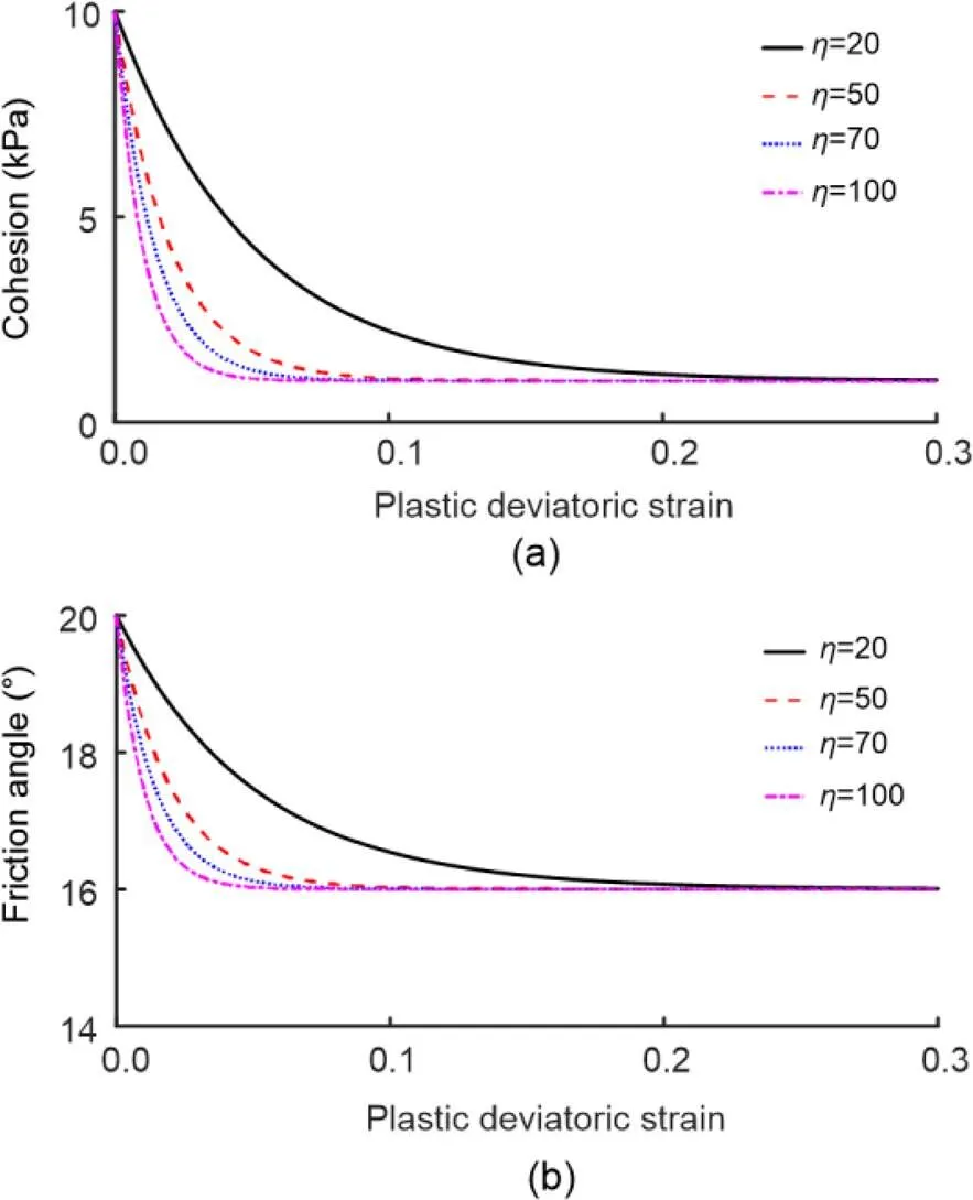
Fig. 8 Strain-softening Mohr-Coulomb model

(a) Cohesion; (b) Friction angle

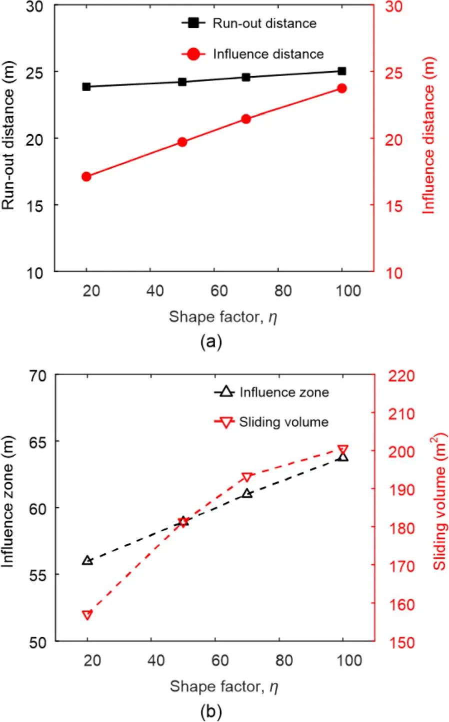
Fig. 9 Calculated post-failure slope features in relation to different shape factors: (a) run-out distance and influence distance; (b) influence zone and sliding volume

3.3 Effects of residual strength

Yerro Colom (2015) reported that the residual strength can also influence the quantitative features of slope failure, but only the influence of residual cohesion on the run-out distance was considered. As proposed by Zhang et al. (2014) and Zhang and Xiao (2019), compared with residual cohesion, the effects of the residual friction angle on the run-out distance are more pronounced. Therefore, in this part, the effects of residual cohesion and friction angle will be studied systematically. The ratios of the residual strength to the peak strength for cohesion and the friction angle were set to 0.5, 0.1, 0.0, and 0.9, 0.8, 0.5, respectively. For the other soil parameters, refer to Table 1. Nine groups of simulations were conducted. The strength reduction shape factorwas set to 20. The strain-softening models are shown in Fig. 10.

Fig. 11 shows that the larger the residual cohesion and friction angle, the smaller the post-failure features of slopes observed. The major reason is that a slope will fail when the driving force exceeds the resistant force. Once soil mass starts to slide, the magnitude of the driving force minus the resistant force determines the eventual deposition of the soil mass. In the current study, the resistant force was composed mainly of the magnitude of the residual shear strength. That meant the post-failure behavior of the slope could be significantly affected by the residual strength.

While the residual cohesion has little impact on the influence distance, it can have a greater effect on the run-out distance. In terms of the residual friction angle, it can considerably affect these four post-failure consequences. Note that the above observation was made based on the slope geometry and soil properties in this analysis. As shown by Hungr et al. (2014), a sandy slope generally experiences a shallow failure, while a clay or silty slope is subjected to a rotational, compound, or planar slide. This is mainly because the frictional resistance is stress dependent, while the cohesion is not. The outcome might also depend on the size of the slope.

4 Probabilistic analysis and results

The mesh size affects not only the calculated FOS of the slope, but also the simulated post-failure behavior of the slope in MPM. Additionally, the strength reduction shape factor and the residual strength can affect the calculated post-failure consequences of the slope. Based on the above analysis, in this section, the mesh size and shape factor were set to 0.5 m and 20, respectively, to investigate slope stability in spatially variable soils and post-failure behavior considering different cross-correlations ofand. The size and geometry of the slope model were the same as shown in Fig. 3. The soil parameters were summarized in Table 2. Among them,andboth followed lognormal distributions with prescribed means and COVs.

Fig. 10 Strain-softening Mohr-Coulomb model under different residual strengths

(a) Cohesion; (b) Friction angle

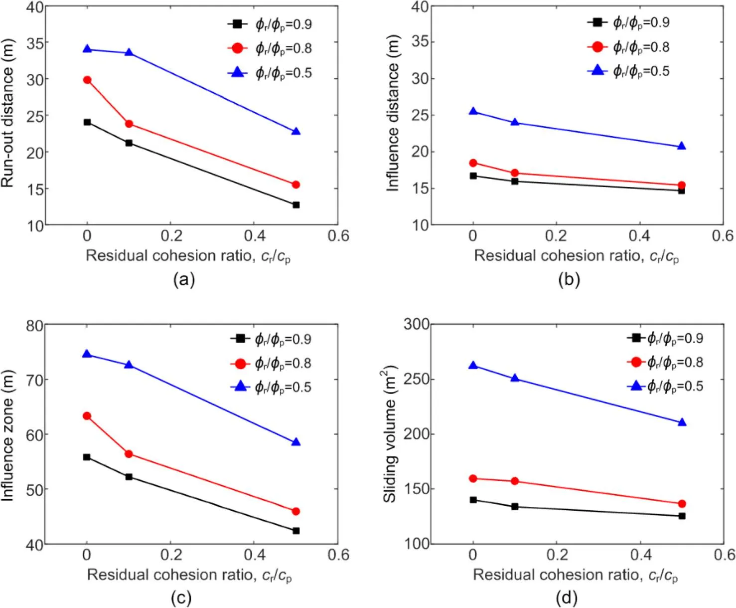
Fig. 11 Results of simulations under different residual strength ratios

(a) Run-out distance; (b) Influence distance; (c) Influence zone; (d) Sliding volume

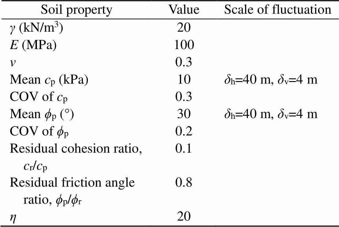
Table 2 Deterministic and spatially variable soil properties

4.1 Convergence analysis

In MCS, choosing a proper number of simulation runs is very important. If the number of simulations is very large, it will be time-consuming, but if relatively few, it will not lead to statistically reliable results.

Fig. 12 plots the mean of run-out distance and its standard deviation against the number of simulations. Clearly, when the number of simulations increases to 100, both the mean of the run-out distance and its standard deviation tend to converge. Therefore, the number of MCS realizations was set to 100 in this study. For each simulation, the average CPU time was about 0.5 h.

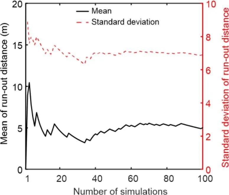
Fig. 12 Mean of run-out distance and its standard deviation in relation to the number of simulations (ρc,ϕ=0.0)

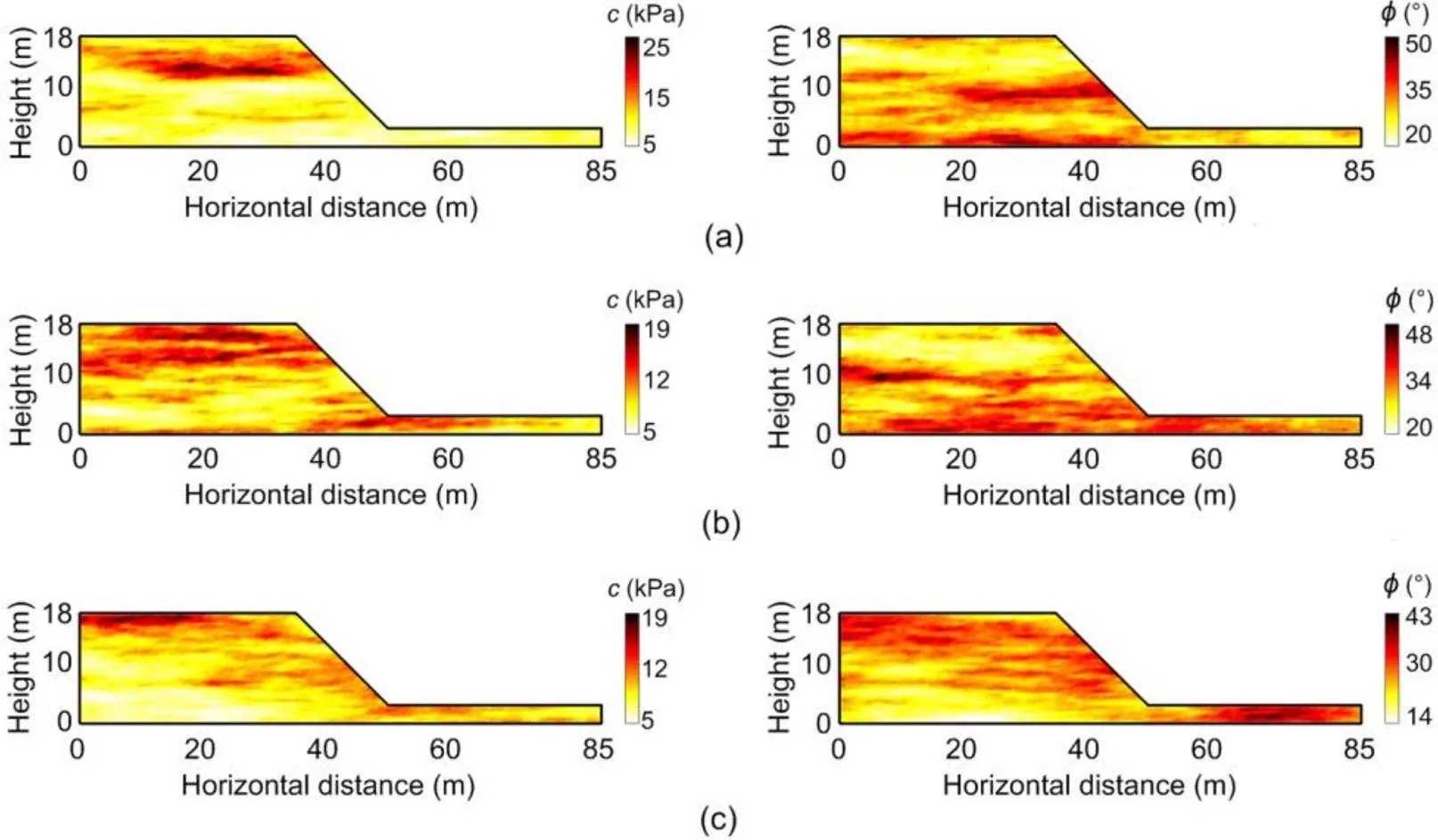
Fig. 13 Three examples of cross-correlated c–ϕ random fields (peak strength)

(a)ρ,ϕ=−0.5; (b)ρ,ϕ=0.0; (c)ρ,ϕ=0.5

4.2 Simulation results

According to the soil parameters in Table 2, the slope is statically stable when ignoring the spatial variability of soil properties. In this part, five different values ofρ,ϕ(−0.5, −0.2, 0.0, 0.2, and 0.5) were chosen such that the effects ofρ,ϕonfand post-failure behavior of slopes could be studied. Accordingly, the risk of slope failure could be assessed quantitatively. Three examples of cross-correlated–random fields (peak strength) under differentρ,ϕvalues are shown in Fig. 13.

Fig. 14 shows thefcalculated by RMPM and RFEM under different cross-correlation coefficients. In FEM calculation, when the numerical algorithm cannot converge and nodal displacement dramatically increases, slope “failure” is said to have occurred (Griffiths and Lane, 1999). In RMPM simulation, the calculated slope failure probabilityfincreases with an increase in the cross-correlation coefficient(fincreases from 0.29 to 0.40 whenρ,ϕincreases from −0.5 to 0.5). These results are consistent with previous findings (Cho, 2010; Li et al., 2015; Liu et al., 2017; Wang MX et al., 2020). Note that both RMPM and RFEM provide similarfvalues, which is reasonable considering that MPM can be considered as the FEM when simulating small deformation problems. It also indicates that the selected 0.4 m of displacement-based failure criterion is reasonable for RMPM simulation.

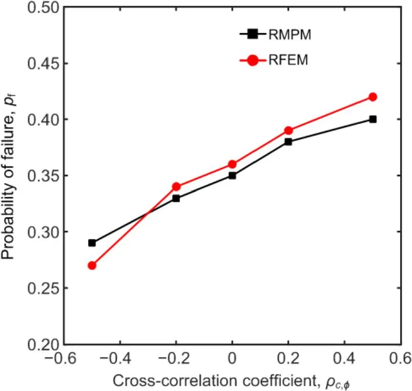
Fig. 14 Probability of failure calculated by RMPM and RFEM under different cross-correlation coefficients

Fig. 15 shows a case of progressive slope failure usingρ,ϕ=0.5. At the time of=1.5 s (Fig. 15a), a shear band begins to form within the soil slope, and slope failure is initiated. At=2.5 s, the shear band is intensified, with deviatoric plastic strain up to 100%–200%, and the slip surface extends from the crest to the toe. Figs. 15c and 15d show that a large deformation develops progressively within the slope as the slip surface extends deeper into the base and further from the crest, while the sliding mass continues to flow till it reaches its final deposition profile at=10 s. The simulated run-out distance and influence distance were 19.97 m and 15.23 m, respectively (Fig. 15d).

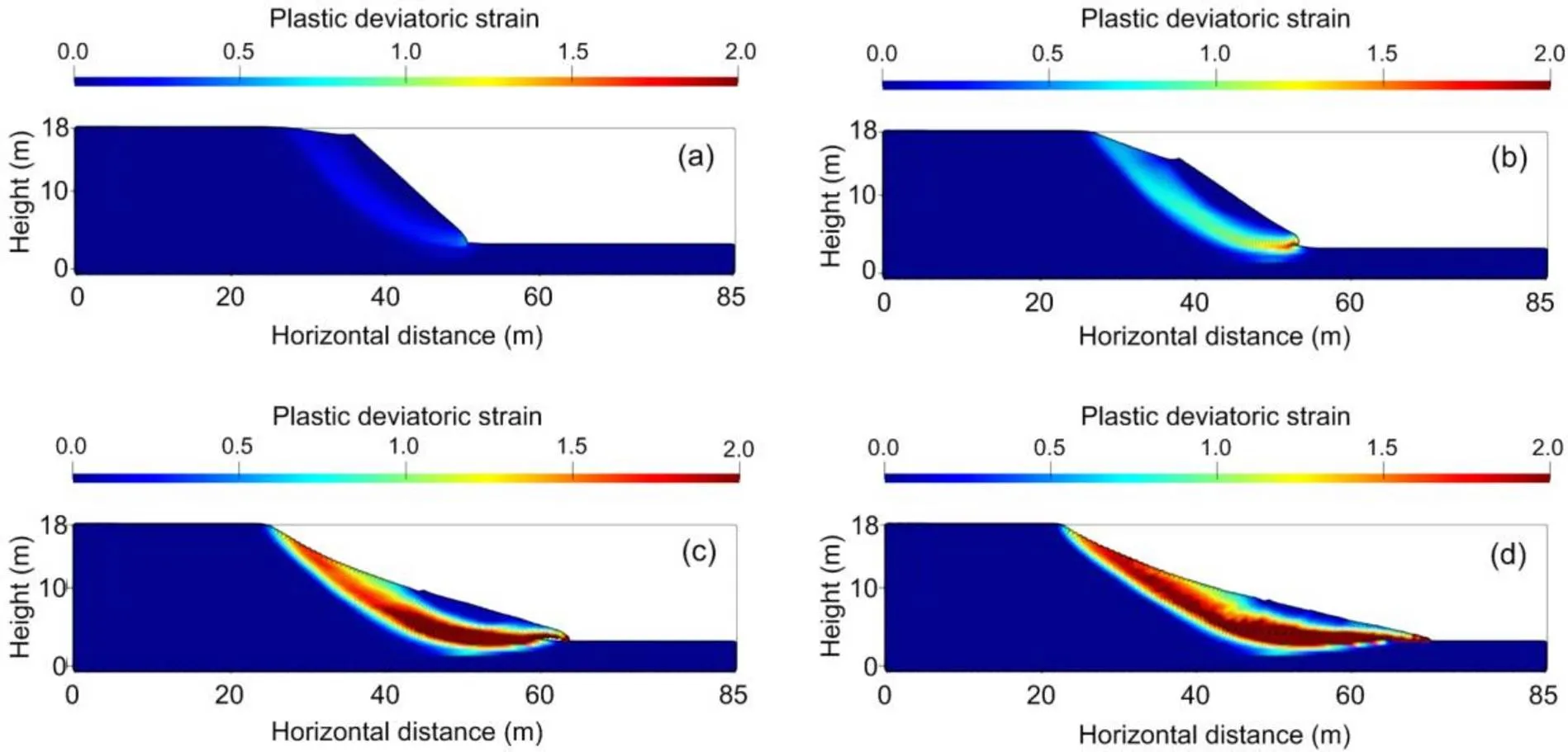
Fig. 15 An example of progressive slope failure

(a)=1.5 s; (b)=2.5 s; (c)=4.5 s; (d)=10 s

In Figs. 16a and 16b, the mean values of slope post-failure consequences (i.e. run-out distance, influence distance, influence zone, and sliding volume) increase only slightly (<5%) with the cross-correlation coefficientρ,ϕ. Here, two different failure consequence indicators (i.e. influence zone and sliding volume) were used to calculate the slope failure risk. These two risk indicators show a consistent trend with the probability of failure curve. Both increased withρ,ϕ, and the largest cross-correlation coefficient resulted in the highest risk.

Statistical distributions of four failure consequences are illustrated in Fig. 17 using two differentρ,ϕvalues for the failed slope cases (non-failure cases are not included), whereρ,ϕ=−0.5 and 0.5 correspond to cases with the lowest and the highest risks, respectively. When theρ,ϕincreases from −0.5 to 0.5, the scattering of the influence zone and sliding volume of the slopes becomes larger. In addition, mean values of all the post-failure measures are slightly larger whenρ,ϕ=0.5, which is consistent with Figs. 16a and 16b.

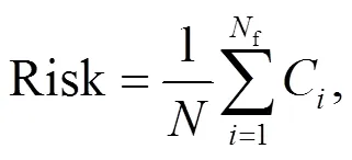
Fig. 18 (p.867) further compares the results of simulation by RMPM and RFEM. The risk was calculated by multiplying the failure probability by the sliding volume associated with each failure. Although the probability of failure calculated by these two methods was similar (Fig. 14), the calculated sliding volume and risk of failure by RFEM were considerably smaller than those by RMPM. Specifically, the sliding volume calculated by RMPM was about 1.5 times that of RFEM (Fig. 18a). The discrepancy is due mainly to differences in the numerical algorithms. In FEM, numerical non-convergence and slope failure occur simultaneously. In other words, FEM cannot simulate the full large deformation process of slope failure due to mesh distortion, and the program will terminate prematurely, resulting in an underestimated sliding volume and a lower risk (Fig. 18b). On the other hand, the MPM combines the Eulerian and Lagrangian methods, and therefore has great advantages for simulating the whole process of slope failure.

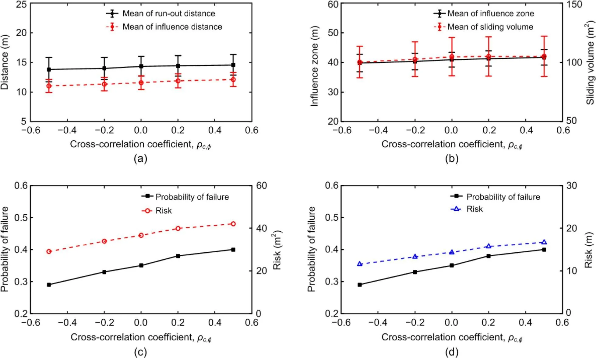
Fig. 16 Post-failure features and risk of failure under different ρc,ϕ values

(a) Run-out distance and influence distance; (b) Influence zone and sliding volume; (c) Probability of failure and risk indicator (by sliding volume); (d) Probability of failure and risk indicator (by influence zone)

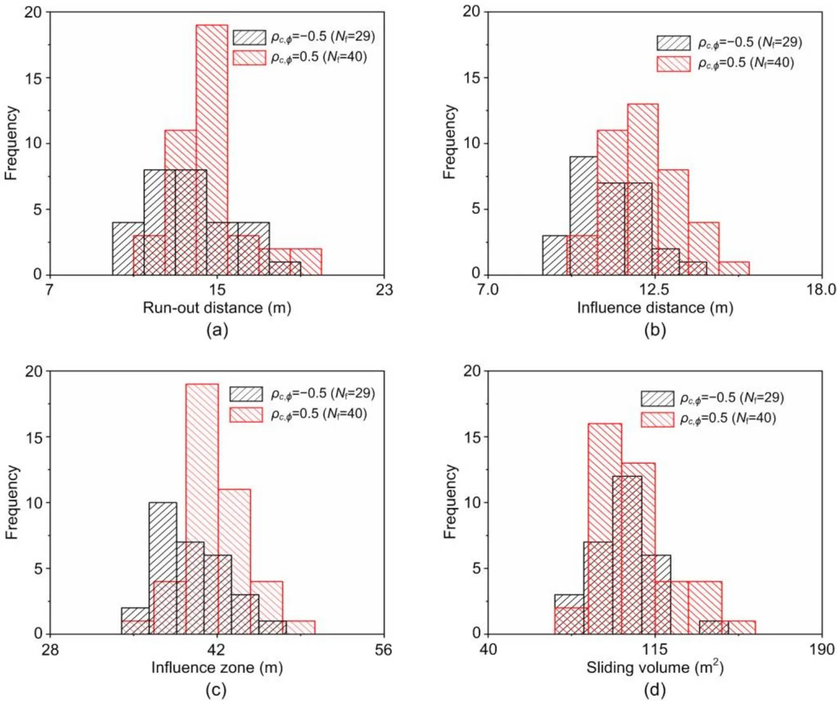
Fig. 17 Distribution of post-failure features for two ρc,ϕ slope cases

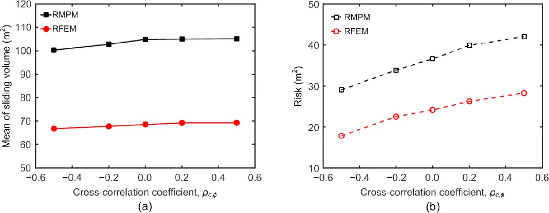
Fig. 18 Calculated sliding volume and risk of failure by RMPM and RFEM

(a) Sliding volume; (b) Risk of failure

Furthermore, compared with the post-failure behavior of slopes, the effects ofρ,ϕonfwere more significant in both the RMPM and RFEM calculations. Although the soil shear strength parameters were spatially variable in the current study, they had more effects on the spatial distribution of shear strength than the magnitude of the shear strength. Generally, the slope seeks the weakest path to fail. That is why there is a greater impact onfthan on the post-failure consequences.

5 Conclusions

This study aimed to investigate the impacts of the cross-correlation betweenandon the post-failure behavior of slopes and risk assessment. The differences in the means of post-failure features under differentρ,ϕvalues were negligible, while the probability of failure was influenced to a relatively large degree. Moreover, the effects of the influencing factors (i.e. mesh size, strength reduction shape factor, and residual strength) on slope stability and post-failure features were analyzed by MPM. The main conclusions can be drawn as follows:

1. RMPM simulation showed that the slope failure probability is greatly influenced by the cross-correlation coefficient ofand. A positiveρ,ϕresults in a larger failure probability than a negativeρ,ϕ. On the other hand, an increase inρ,ϕincreases the post-failure consequences of the failed slopes only slightly (by 5%–10%).

2. MPM suffers from mesh-dependency when using a strain-softening model to simulate slope failure. Therefore, the mesh size has a significant impact on the simulation results, and a mesh sensitivity study should be conducted. In this study, the calculated FOS and post-failure features tended to converge when a mesh size smaller than 0.5 m was used. As a finer mesh size can significantly increase computational time, in this study, a mesh size of 0.5 m was used by considering both computational accuracy and efficiency.

3. When the mesh size is fixed, all post-failure features increase with the strength reduction shape factor. An increase in the residual cohesion and friction angle will result in a reduced run-out distance, influence distance, influence zone, and sliding volume. Moreover, compared with the residual cohesion, the residual friction angle has a more pronounced influence on the slope post-failure consequences in terms of the slope geometry and soil properties employed.

4. The probabilities of slope failure calculated by RMPM and RFEM were quite similar, which indicates that both methods are capable of handling relatively small deformations upon triggering of a slope failure. The displacement-based failure criterion (0.4 m) seems to be reasonable for MPM analysis. However, RFEM considerably underestimates the post-failure features and risks associated with slope failure compared with RMPM, because FEM will end in non-convergence due to mesh distortion. The entire progressive slope failure process can be simulated using RMPM.

The SOFs of soil properties may also affect the post-failure behavior of slopes. Furthermore, rotated anisotropic soil fabric can be observed in nature due to soil deposition, weathering, or filling. The effects of these features on the post-failure behavior of slopes also need to be investigated in the future.

Contributors

Chuan-xiang QU: conceptualization, formal analysis, investigation, software, writing–original draft, writing–review & editing. Gang WANG: conceptualization, methodology, funding acquisition, supervision, validation, writing–review & editing. Ke-wei FENG: methodology, software, validation. Zhen-dong XIA: validation, software.

Conflict of interest

Chuan-xiang QU, Gang WANG, Ke-wei FENG, and Zhen-dong XIA declare that they have no conflict of interest.

Abbo AJ, Sloan SW, 1995. A smooth hyperbolic approximation to the Mohr-Coulomb yield criterion., 54(3):427-441.https://doi.org/10.1016/0045-7949(94)00339-5

Bandara S, Soga K, 2015. Coupling of soil deformation and pore fluid flow using material point method., 63:199-214.https://doi.org/10.1016/j.compgeo.2014.09.009

Bandara S, Ferrari A, Laloui L, 2016. Modelling landslides in unsaturated slopes subjected to rainfall infiltration using material point method., 40(9): 1358-1380.https://doi.org/10.1002/nag.2499

Cheng HZ, Chen J, Chen RP, et al., 2018. Risk assessment of slope failure considering the variability in soil properties., 103:61-72.https://doi.org/10.1016/j.compgeo.2018.07.006

Cho SE, 2010. Probabilistic assessment of slope stability that considers the spatial variability of soil properties., 136(7):975-984.https://doi.org/10.1061/(ASCE)GT.1943-5606.0000309

Feng K, Wang G, Huang D, et al., 2021a. Material point method for large-deformation modeling of coseismic landslide and liquefaction-induced dam failure., 150:106907.https://doi.org/10.1016/j.soildyn.2021.106907

Feng K, Huang D, Wang G, 2021b. Two-layer material point method for modeling soil–water interaction in unsaturated soils and rainfall-induced slope failure., 16:2529-2551.https://doi.org/10.1007/s11440-021-01222-9

Griffiths DV, Lane PA, 1999. Slope stability analysis by finite elements., 49(3):387-403.https://doi.org/10.1680/geot.1999.49.3.387

Huang D, Wang G, Du C, et al., 2020. An integrated SEM-Newmark model for physics-based regional coseismic landslide assessment., 132:106066.https://doi.org/10.1016/j.soildyn.2020.106066

Huang J, Lyamin AV, Griffiths DV, et al., 2013. Quantitative risk assessment of landslide by limit analysis and random fields., 53:60-67.https://doi.org/10.1016/j.compgeo.2013.04.009

Hungr O, Leroueil S, Picarelli L, 2014. The Varnes classification of landslide types, an update., 11(2):167-194.https://doi.org/10.1007/s10346-013-0436-y

Li DQ, Jiang SH, Cao ZJ, et al., 2015. A multiple response-surface method for slope reliability analysis considering spatial variability of soil properties., 187:60-72.https://doi.org/10.1016/j.enggeo.2014.12.003

Li DQ, Xiao T, Cao ZJ, et al., 2016. Enhancement of random finite element method in reliability analysis and risk assessment of soil slopes using subset simulation., 13(2):293-303.https://doi.org/10.1007/s10346-015-0569-2

Liu LL, Cheng YM, Zhang SH, 2017. Conditional random field reliability analysis of a cohesion-frictional slope., 82:173-186.https://doi.org/10.1016/j.compgeo.2016.10.014

Liu X, Wang Y, Li DQ, 2019. Investigation of slope failure mode evolution during large deformation in spatially variable soils by random limit equilibrium and material point methods., 111:301-312.https://doi.org/10.1016/j.compgeo.2019.03.022

Liu X, Wang Y, Li DQ, 2020. Numerical simulation of the 1995 rainfall-induced Fei Tsui Road landslide in Hong Kong: new insights from hydro-mechanically coupled material point method., 17(12):2755-2775.https://doi.org/10.1007/s10346-020-01442-2

Ng CWW, Qu CX, Cheung RWM, et al., 2021. Risk assessment of soil slope failure considering copula-based rotated anisotropy random fields., 136:104252.https://doi.org/10.1016/j.compgeo.2021.104252

Oliver J, Huespe AE, 2004. Continuum approach to material failure in strong discontinuity settings., 193(30-32): 3195-3220.https://doi.org/10.1016/j.cma.2003.07.013

Soga K, Alonso E, Yerro A, et al., 2016. Trends in large-deformation analysis of landslide mass movements with particular emphasis on the material point method., 66(3):248-273.https://doi.org/10.1680/jgeot.15.LM.005

Sulsky D, Chen Z, Schreyer HL, 1994. A particle method for history-dependent materials., 118(1-2):179-196.https://doi.org/10.1016/0045-7825(94)90112-0

Sulsky D, Zhou SJ, Schreyer HL, 1995. Application of a particle-in-cell method to solid mechanics., 87(1-2):236-252.https://doi.org/10.1016/0010-4655(94)00170-7

Vanmarcke EH, 1983. Random Fields: Analysis and Synthesis. MIT Press, Cambridge, USA.

Wang B, Vardon PJ, Hicks MA, 2016a. Investigation of retrogressive and progressive slope failure mechanisms using the material point method., 78:88-98.https://doi.org/10.1016/j.compgeo.2016.04.016

Wang B, Hicks MA, Vardon PJ, 2016b. Slope failure analysis using the random material point method., 6(2):113-118.https://doi.org/10.1680/jgele.16.00019

Wang B, Vardon PJ, Hicks MA, 2018. Rainfall-induced slope collapse with coupled material point method., 239:1-12.https://doi.org/10.1016/j.enggeo.2018.02.007

Wang MX, Tang XS, Li DQ, et al., 2020. Subset simulation for efficient slope reliability analysis involving copula-based cross-correlated random fields., 118:103326.https://doi.org/10.1016/j.compgeo.2019.103326

Wang MY, Liu Y, Ding YN, et al., 2020. Probabilistic stability analyses of multi-stage soil slopes by bivariate random fields and finite element methods., 122:103529.https://doi.org/10.1016/j.compgeo.2020.103529

Wang Y, Qin ZW, Liu X, et al., 2019. Probabilistic analysis of post-failure behavior of soil slopes using random smoothed particle hydrodynamics., 261:105266.https://doi.org/10.1016/j.enggeo.2019.105266

Yerro A, Alonso EE, Pinyol NM, 2015. The material point method for unsaturated soils., 65(3):201-217.https://doi.org/10.1680/geot.14.P.163

Yerro Colom A, 2015. MPM Modelling of Landslides in Brittle and Unsaturated Soils. PhD Thesis, Universitat Politècninca de Catalunya, Barcelona, Spain.

Yin YP, Li B, Wang WP, et al., 2016. Mechanism of the December 2015 catastrophic landslide at the Shenzhen landfill and controlling geotechnical risks of urbanization., 2(2):230-249.https://doi.org/10.1016/J.ENG.2016.02.005

Zhang WJ, Xiao DQ, 2019. Numerical analysis of the effect of strength parameters on the large-deformation flow process of earthquake-induced landslides., 260:105239.https://doi.org/10.1016/j.enggeo.2019.105239

Zhang YB, Xu Q, Chen GQ, et al., 2014. Extension of discontinuous deformation analysis and application in cohesive-frictional slope analysis., 70:533-545.https://doi.org/10.1016/j.ijrmms.2014.06.005

Zhu H, Zhang LM, 2013. Characterizing geotechnical anisotropic spatial variations using random field theory., 50(7):723-734.https://doi.org/10.1139/cgj-2012-0345

https://doi.org/10.1631/jzus.A2100196

P642.22

Apr. 24, 2021;

May 29, 2021;

Oct. 19, 2021

*Project supported by the Fund of Hong Kong Research Grants Council (RGC) (No. 16214519), China

© Zhejiang University Press 2021