An investigation into intermittent electrification strategies and an analysis of resulting CO2 emissions using a high-fidelity train model

Bilal M. Abdurahman• Tim Harrison• Christopher P. Ward•William J. B. Midgley

Abstract A near-term strategy to reduce emissions from rail vehicles, as a path to full electrification for maximal decarbonisation, is to partially electrify a route, with the remainder of the route requiring an additional self-powered traction option. These rail vehicles are usually powered by a diesel engine when not operating on electrified track and are referred to as bi-mode vehicles.This paper analyses the benefits of discontinuous electrification compared to continuous electrification using the CO2 estimates from a validated high-fidelity bi-mode(diesel-electric)rail vehicle model. This analysis shows that 50% discontinuous electrification provides a maximum of 54% reduction in operational CO2 emissions when compared to the same length of continuously electrified track. The highest emissions savings occurred when leaving train stations where vehicles must accelerate quickly to line speed. These results were used to develop a linear regression model for fast estimation of CO2 emissions from diesel running and electrification benefits.This model was able to estimate the CO2 emissions from a route to within 10%of that given by the high-fidelity model. Finally, additional considerations such as cost and the embodied CO2 in electrification infrastructure were analysed to provide a comparison between continuous and discontinuous electrification.Discontinuous electrification can cost up to 56% less per reduction in lifetime emissions than continuous electrification and can save up to 2.3 times more lifetime CO2 per distance electrified.

Keywords Railway electrification ∙CO2 reduction ∙Discontinuous electrification ∙Bi-mode rail vehicle

1 Introduction

In order to achieve the net-zero carbon emissions target by 2050,the UK government aims to stop the sale of internalcombustion-only cars by 2035 and remove all diesel-only railway traction by 2040 [1, 2]. The UK’s commitment to decarbonisation is in conjunction with the global effort to reduce carbon emissions and is supported by its rail transport sector [3].

Currently,about 38%of UK’s rail network is electrified and 70% of all passenger rail vehicles are electric [4].Decarbonisation may require most, if not all, of the networks to be electrified since electrified traction produces the lowest operational carbon emissions for rail transport[5].Current decarbonisation plans suggest electrification of 85% of the remainder of the network, with battery and hydrogen propulsion used for 8% and 5% respectively,leaving 2% with no clear electrification business case[3, 6].

Electric traction on more intensively used sections of the routes also provides the least whole-life carbon footprint,and delivers faster, more reliable, quieter services and is less polluting than diesel[3].In addition,for long-distance high-speed and rail freight services on the UK railway,electrification is the only suitable option compared to hydrogen and battery powered technologies since only electric traction can provide the performance necessary to deliver services in accordance with operational requirements [6]. Electric trains also provide lower cumulative emissions than hydrogen trains [7].

If a given route is to be fully electrified, which can be costly at £1 M/STK (single-track kilometre) to £2.5 M/STK [6], and before this electrification is completed other modes of rail transport such as hydrogen, battery and bimode vehicles, which run either on diesel or on power supplied by overhead line equipment (OLE) when it is available, offer short-term carbon-reduction solutions.

Reducing energy consumption in railways directly leads to reduction in CO2emissions, and previous research has looked at driver interventions, which can reduce the total energy consumption by up to 20% [9, 10]. Operational energy consumption (the energy consumption of a vehicle in operation rather than its embodied energy) of a hydrogen-hybrid powered train has been studied in[11],and Ref.[8]presents that of diesel,electric and bi-mode trains.Both works considered high-level models rather than the more detailed component-level model employed here. The latter also only considered constant vehicle operational speed without acceleration or deceleration. In terms of energy efficiency, previous studies in this area have focussed on high-level calculations and lower speed rail vehicle behaviour [12, 13].

Most of the electrified mainline UK rail network uses OLE that is energised at 25 kV AC, the remainder uses 750 V DC third-rail electrification. This paper focuses on 25 kV OLE as this comprises the larger proportion (68%)of the UK’s network [14].

Continuous electrification has been necessary to avoid prolonged loss of power supply to solely electric trains[15]. Bi-mode electric/diesel trains have recently become available, reducing the use of diesel trains on routes that are partly electrified, and opening up the possibility of discontinuous electrification. Continuous electrification presents a challenge if the route includes multiple tunnels and bridges that may require raising or lowering the tracks,or are laid on the side of hills and tight corners [16],increasing the cost of electrification significantly. In such cases,discontinuous electrification is more suitable and can offer a better business case based upon capital cost considerations. Discontinuously or intermittently electrified track is defined here as an electrified track that has one or more unelectrified sections.

There is very limited prior research that has investigated electrification with high-definition vehicle models. In[16],an electric multiple unit (EMU) train with modest energy storage device was simulated and able to complete a 5-km non-electrified route with sufficient performance. A feasibility of discontinuous electrification over the 7-km-long Severn Tunnel was studied in [15] where both diesel and electric trains were able to complete the journey. The Severn Tunnel was fully electrified in 2020.

The novelty of this paper is in its utilisation of a validated high-fidelity bi-mode rail vehicle model to investigate the benefits of discontinuous and continuous electrification on the CO2emissions of rail transport.Section 2 summarises the construction and validation of the high-fidelity vehicle model. Section 3 uses this model to investigate the emissions from an example route and develop a method for near-optimal discontinuous electrification, comparing this to continuous electrification. Section 4 develops a linear regression model to estimate CO2emissions from a given route and compares the discontinuous electrification suggested by this model to the results from the high-fidelity model. Section 5 expands the problem to include the effects of cost and embedded carbon dioxide emissions on the justification for discontinuous and continuous electrification.

2 Rail vehicle model

The work reported here extends and improves upon the model initially described in [17]. An overview of this model is given in Fig. 1. The model has independent modular components that can be swapped for another of the same type,similar to functional mock-up units(FMUs)[18].

The rail vehicle investigated is the Hitachi AT300 product family (Class 800, 801 and 802, here denoted as 80x) of trains currently being introduced onto the UK rail network.Class 800 and 802 are a 5 or 9 car bi-mode(25 kV electric/diesel) trains capable of operating at up to 225 km/h [19].Class 801 are similar but are 25 kV electric trains with only a single engine-generator set for emergency power and lowspeed movement away from OLE.The 5-car version of Class 802 is used in this study.The energy storage device was not implemented because it is not present in bi-mode trains,but due to the modular characteristics of the model,it can easily be added.

2.1 Timetable and routes

The route studied in this paper is London Paddington to Plymouth via Westbury (shown in Fig. 2), with timetable data obtained from OpenTrainTimes [20]. The speed limits on the route were taken from the Network Rail’s national electronic sectional appendices for June 2019 [21].

2.2 Train driver

The train driver model is responsible for accelerating up to and maintaining the speed limit and decelerating no faster than a given deceleration rate.The driver controller G(s )is given by

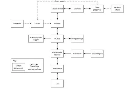
Fig. 1 Components of the train model. OLE—overhead line equipment [17]

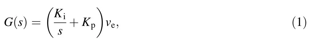
where s is the Laplace operator,Kiand Kpare integral and proportional coefficients of 0.5 Am-1and 550 Asm-1,respectively, and ve＝vd-v is the velocity error with v and vdbeing the actual and desired train velocities. v is obtained by integrating the vehicle equations of motion,while vdis calculated in small increments by the timetable block using the station positions and speed limit data.Then,G(s )produces the desired current to the motors and generators using ve.

2.3 Train dynamics and properties

The train parameters and properties were obtained from publicly available information [19] and are given in Table 1. A 40% passenger loading, which is typical in operational calculations for this route,with each passenger weighing 90 kg was used in all simulations [22].

The acceleration of the train is determined by the sum of the forces acting on it, which is given by

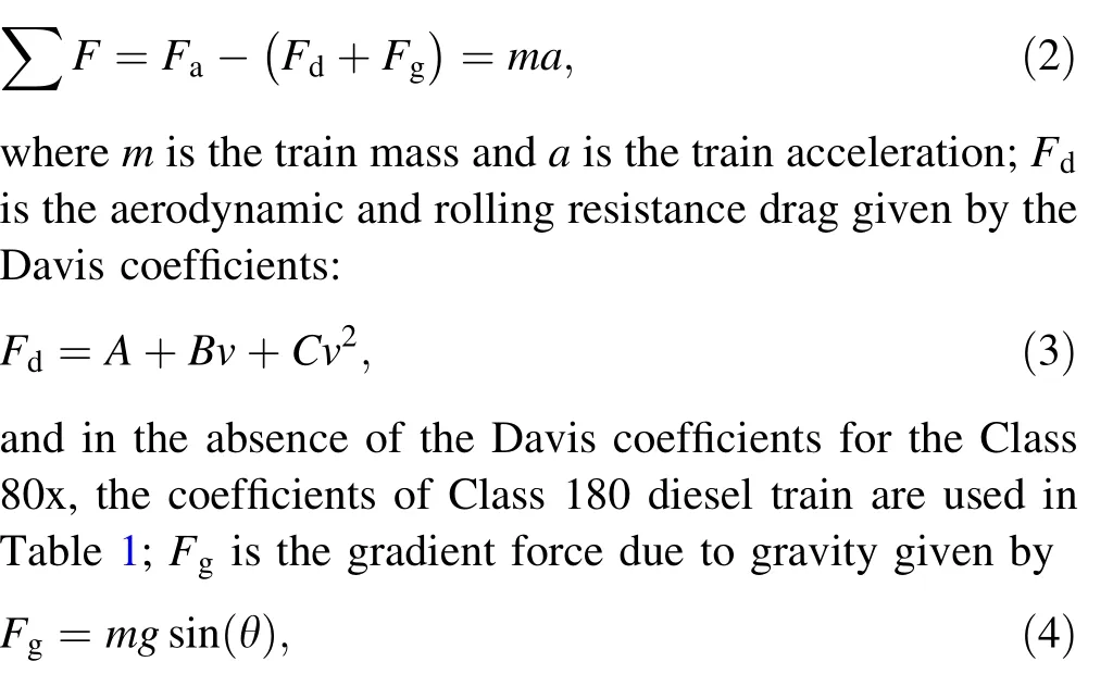
where m is the train mass, g is the acceleration due to gravity(9.8 ms-2),and θ is the angle from the sea level to the forward inclination of the track. The force available to accelerate the train is the traction force from electric motors Faminus the drag and gradient forces.

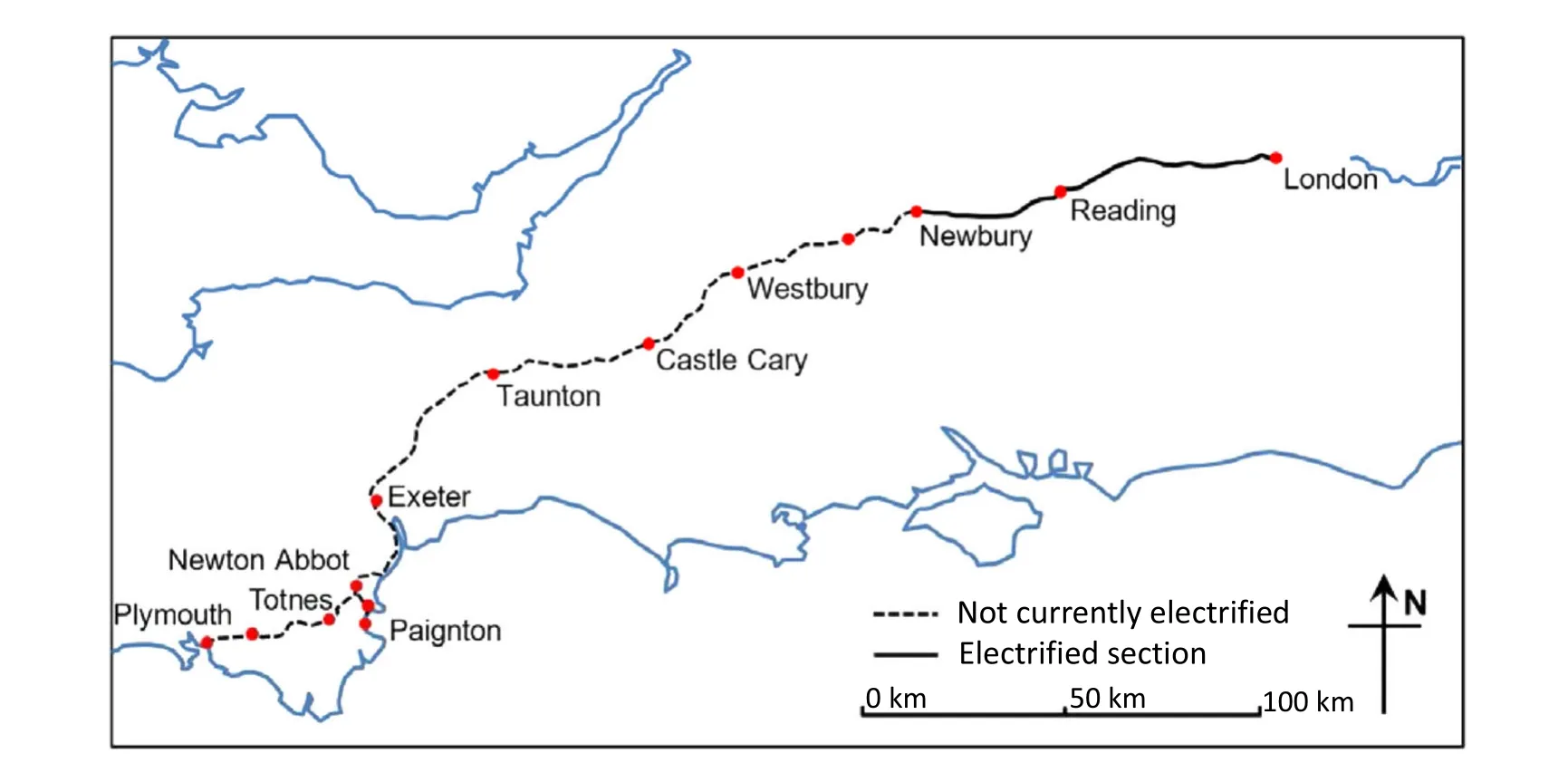
Fig. 2 London to Plymouth and Paignton route [17]

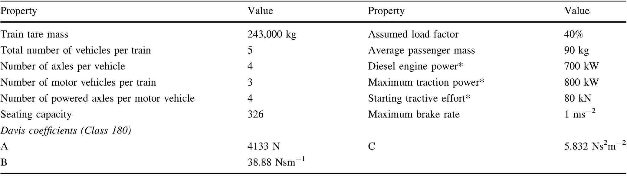
Table 1 Model input parameters for the Class 80x 5-car train [17, 19, 23]

2.4 Deceleration and braking

The Class 80x trains use electro-dynamic braking,blended with friction braking at low speeds (this blending is not modelled in detail in the simulation). In electric mode, the power generated is fed back into the OLE at an assumed 40% regeneration efficiency. In diesel mode, the energy is dissipated in resistors on the roof of the vehicle.The target deceleration rate for slowing into stations of 0.4 ms-2was used.

2.5 Auxiliary power requirements

Based on discussions with rail operators,the so-called hotel load—the power required to run air compressors, heating,lighting and air conditioning—was set to 20 kW per train.In some environments, this can be up to 50 kW per train for modern units, but depends on environmental and loading conditions [24].

2.6 Diesel engine and generator

The diesel engine model used in this simulation was based on a model of a heavy goods vehicle [25] scaled to match the specifications of the class 80x train engines[26].More information on the dynamics of the engine/generator set is available in [17].

2.7 Overhead line equipment (OLE) and bi-mode operation

It is assumed that the OLE functions as a perfect power source,supplying sufficient power for the electric motors to run at their maximum power output. It is possible that power from the OLE can be restricted, due to the number of trains on a single section of OLE. This has not been modelled here,but the model allows this to be incorporated through a simple power limit.When there is OLE available, the desired power to the motors and auxiliaries are provided by the OLE rather than the diesel engine/generator set. When switching to nonpowered sections of track, the engine/generator set starts immediately and provides the desired power.

2.8 Model validation

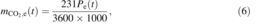
The energy usage and CO2emissions predicted by the model were validated using data gathered during a day of testing in 2020. Example validation plots are given in Fig. 3. In this case, the in-service train slowed down after Westbury and after Taunton because of speed restrictions.The model gave fuel consumption of 3.27–3.46 L/mile and 0.016–0.017 L/(passenger∙km)—in line with similar rolling stock such as the Class 221 and Class 180. Further details of the validation are given in [17].

3 CO2 emissions

3.1 Model results

Since the section of the route from London Paddington to Newbury had already been electrified, the model was run first in diesel and then in electric mode from Newbury to Plymouth to compare the different CO2footprints of each traction mode. The results of this modelling are given in Fig. 4.

The electrical power use Pe(t) in watts is calculated as

where Pemis the motor electrical power, Pauxis the auxiliary power use,nm＝12 is the total number of motors,Viis the motor input voltage, and imis the single motor current. The traction motor is modelled as a DC motor as given in [17].

The CO2emitted when running on OLE is calculated using 231 g/kWh, the current carbon intensity of the UK’s electricity grid [27]. In this case, the instantaneous CO2in g from electric traction is given by

where mCO2,e(t)is the instantaneous mass of CO2in g from electric traction.

This equation is then integrated over the simulation time to obtain the total CO2emission for a given section or route. As most countries (including the UK) shift towards renewable energy generation, the carbon intensity of the grid will decrease,improving the CO2emissions benefits of rail electrification.

Figure 4 shows that CO2emissions are higher for both traction modes when the vehicle is accelerating or going uphill,as expected.The correlation to uphill cruising mode can be seen at around 160 km into the journey where the train cruises uphill and produces similar CO2as if it were accelerating in non-uphill sections, in both diesel and electric traction. There are also larger differences in CO2emissions for cruising versus acceleration for the train running under electric traction.

3.2 Route analysis

It is clear from Fig. 4 that each part of the route is responsible for differing CO2emissions.The desire to find an optimal discontinuous electrification strategy requires analysis of the CO2over given sections of the route todetermine which have the highest CO2emissions and should therefore be electrified first.

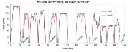
Fig. 3 Example model validation output [17]

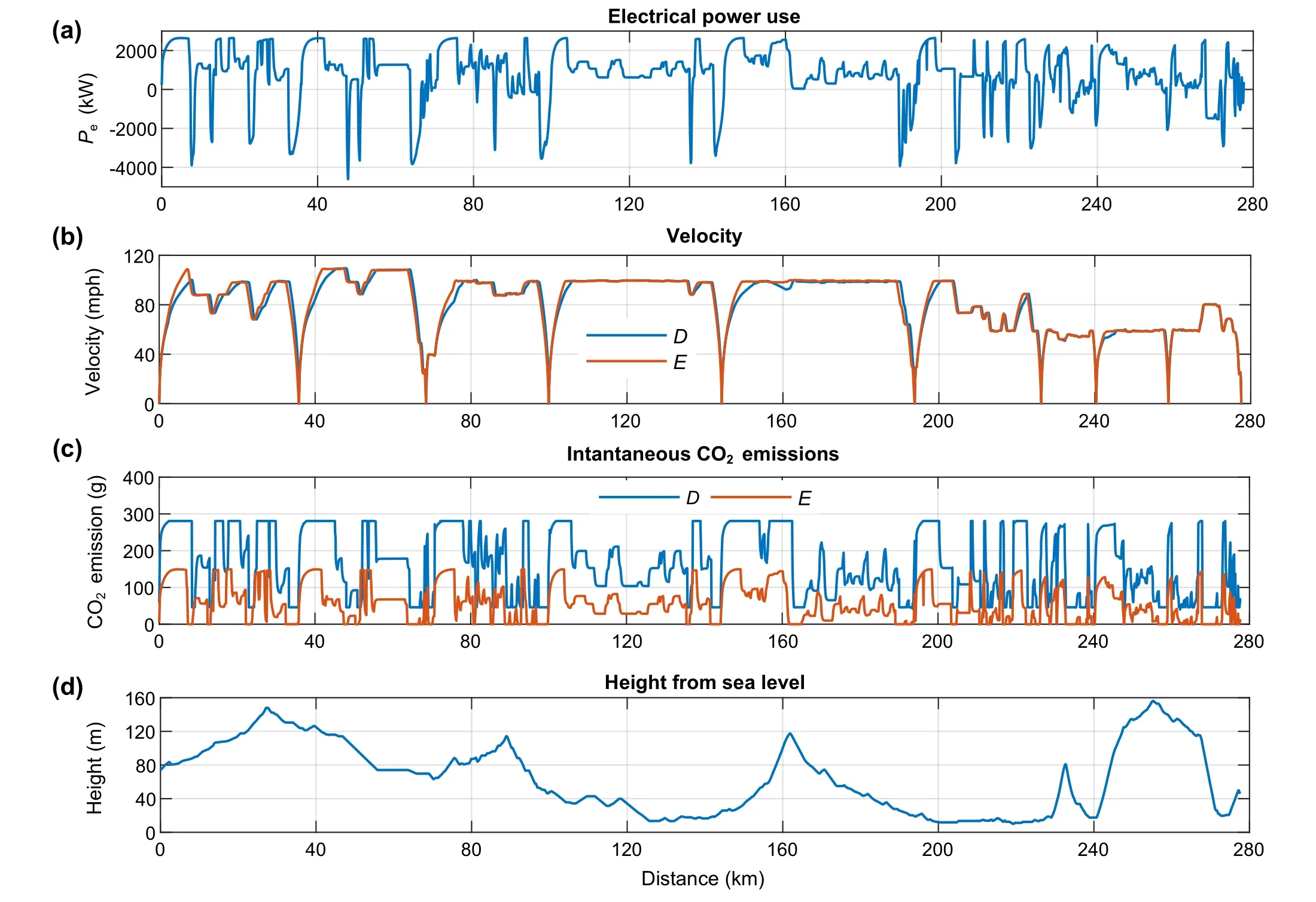
Fig.4 a Train total electrical power use(under electrical traction),b velocity,c instantaneous CO2 emissions on both diesel and electric traction runs, and d vertical profile from Newbury to Plymouth. D = diesel mode, and E = electric mode

To achieve this, the route from London Paddington to Plymouth was divided into 40 sections, each 7 km long.The highest precision would be gained from even shorter sections (e.g. 1-km sections), but it was considered that approximately 7-km sections struck a balance between a minimum viable electrification project and useful conclusions for the optimisation algorithm. The CO2emissions for each of these 40 sections, for both electric and diesel traction, are given in Fig. 5.

Figure 5 shows that the CO2emissions from diesel traction are far greater than those from electric traction, as expected. It also shows peaks in emissions for both diesel and electric traction near stations, where the vehicle uses large amounts of power to accelerate back up to line speed after a station stop. The amount of CO2saved for a given section or percentage of route electrification is computed as follows:

where ΔmCO2is the mass of CO2saved,mCO2,dis the mass of CO2emitted when running on diesel-only,and mCO2,eis the mass of CO2emitted when running on electricity.

If the CO2savings from each sections are sorted from largest to smallest (Fig. 6), then this gives a first-order method for determining which sections should be electrified first.

3.3 Comparison to continuous electrification

It is now possible to compare continuous electrification from Newbury to Plymouth by comparing the amount of CO2saved versus the fraction of the route electrified. As before,the train runs on OLE when it is present and runs on diesel when it is not present, no further changes (for example increasing coasting) have been made.

The results of this comparison are given in Fig. 7.Discontinuous electrification shows diminishing returns as more of the line is electrified, whereas continuous electrification(electrifying incrementally starting from Newbury)shows roughly linear reductions in emissions, with notable jumps at each station.

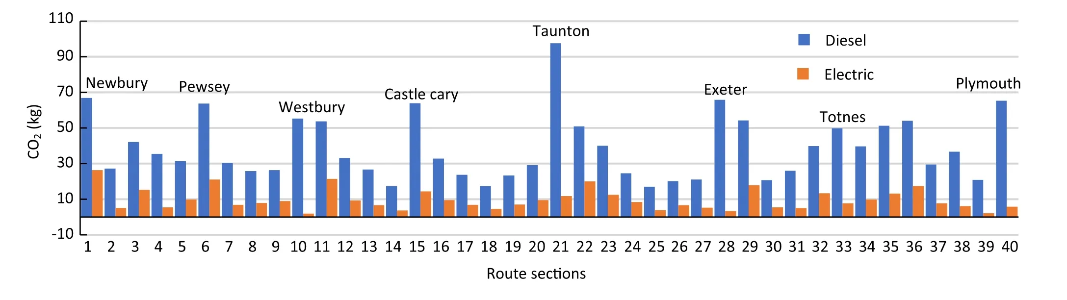
Fig. 5 CO2 emissions from 40 equal 7-km sections of the route from Newbury to Plymouth for diesel and electric traction modes

Fig. 6 Possible CO2 savings from electrification of given sections, sorted by mass of CO2 saved

Figure 7 shows that the maximum saving from discontinuous electrification compared to continuous electrification happens at 50% electrification, saving 282 kg of CO2(a 54% reduction) on a single journey from Newbury to Plymouth. It also shows that, as expected, the difference between the strategies disappears at 100% of electrification. Key extracts from the data in Figs. 6 and 7 are tabulated in Table 2.

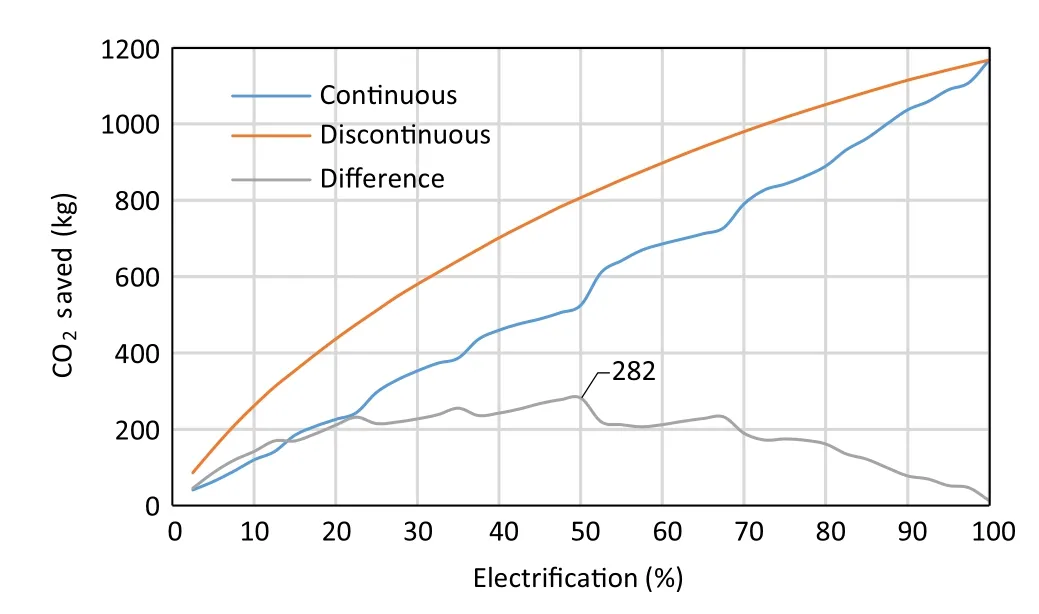
Fig. 7 CO2 savings from electrification between Newbury and Plymouth

Table 2 shows which discontinuous sections are involved at different percentage of route electrification and how many stations this electrification would cover out of the 8 stations identified in Fig. 5. It shows that at 20% of electrification, all stations should be electrified. The table also shows ‘orphan’ sections, whose neighbours are not electrified.For example,at 60%of electrification,only section 40 is ‘orphaned’, which means that the rest of the sections have a minimum continuous length of about 14 km. However, section 40 is at Plymouth station, which means that neighbouring sections are likely to be joined with it as part of an electrification scheme.

Figure 8 gives another perspective on CO2reductions in terms of g/(passenger∙km). It shows that the maximum reduction in normalised CO2from discontinuous electrification compared to continuous electrification is at 22.5%of electrification, with a similar second peak at 47.5%. The maximum in this figure is different to that in Fig. 7,which had its maximum at 50% discontinuous electrification. In Fig. 7, the figures given are total CO2saved, whereas Fig. 8 gives the total CO2emissions per passenger-kilometre for the journey. For example, the maximum CO2saved at 50% in Fig. 7 is the total CO2emitted in the case of continuous electrification minus the total CO2emitted in the case of continuous electrification at 50% ofelectrification, whereas in Fig. 8, the CO2emissions per passenger-kilometre for a continuously electrified (CE)section is determined by

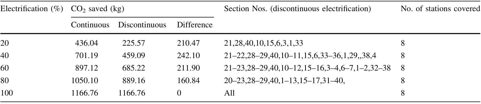
Table 2 Comparison of CO2 savings between discontinuous and continuous electrification from Newbury to Plymouth

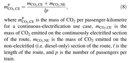
Thus,while Fig. 7 shows the total amount saved,Fig. 8 shows how much CO2is still being emitted(normalised by passenger-kilometres) at a given percentage of route electrification; hence, they have different peaks.

The horizontal dashed red line in Fig. 8 also shows that discontinuous electrification at 32.5%of the route emits the same CO2as continuous electrification at 50%of the route.This means that discontinuous electrification saves 17.5%of the route (48.6 km) from being electrified or approximately £97–243 million in double-track electrification in the short term for the same amount of CO2emissions [6].

Fig. 8 Effect of electrification on normalised CO2 per passengerkilometre

4 Optimal discontinuous electrification

Optimal discontinuous electrification can be looked at as an optimisation problem where the highest CO2emitting sections should be electrified first.These sections are likely to be the high-power sections involving steep vertical climbs,hard acceleration,or high-speed cruising.However,the emissions map (emissions vs power) for the engine[17,25]is highly nonlinear,and thus it is not clear a priori which sections of a given route should be electrified first.

4.1 Electrification approaches

A naı¨ve method to discontinuous electrification might be to electrify the sections of track exiting each station, as the acceleration away from stationary is power intensive, as modelled in [17]. A second method would be to approach the problem as above—running a high-fidelity model over the track to find the sections of track with the greatest CO2emissions and electrifying these sections first.

However, it can be time-consuming to run this highfidelity model over all possible timetabled routes for a given network. Instead, a rule-based discontinuous electrification method can be developed that guarantees nearoptimality of CO2saved per distance of track electrified,without having to run the high-fidelity model.

4.2 Rule-based optimal discontinuous electrification

As mentioned above, engineering judgement suggests that sections of track with high-power demands should be electrified first. However, the vehicle model and CO2emissions map of the rail vehicle are nonlinear and therefore analysis must be undertaken to determine the correlation between emissions and a range of different parameters in order to develop a linear regression model.In this case, the emissions of the rail vehicle under different traction modes were compared against five relevant parameters: instantaneous acceleration, instantaneous velocity,route speed limit,gradient and mechanical power.The results of this correlation are given in Table 3.It showsthat the highest correlation of CO2is with the total traction power demand in both traction modes.

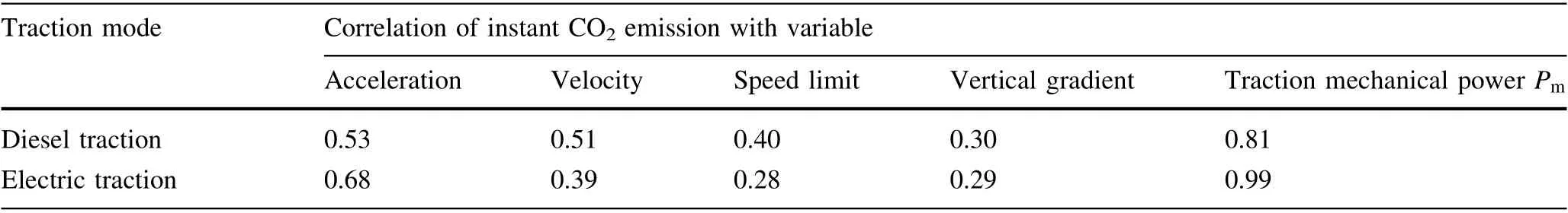
Table 3 Correlation between instantaneous CO2 emission and different variables under different traction modes

For the rule-based analysis, the correlation between instant CO2emission and traction mechanical power Pm(t)is used, which is shown graphically for diesel taction only in Fig. 9. The traction mechanical power is calculated as

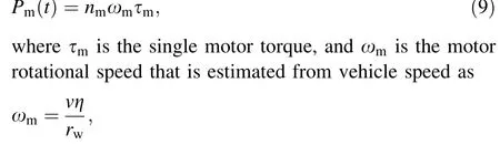
with η and rwbeing the gear ratio and wheel radius,respectively. These parameters are also given in [17].

The figure shows a nonlinear relationship between the instant CO2emission and Pm(t), which is expected since there is a nonlinear relationship between instant CO2emission and the engine power. However, from the correlation,it is possible to investigate whether a linear relation between traction mechanical power and CO2emissions allows the user to estimate optimal discontinuous electrification strategy without having to run the high-fidelity model over a route. In this case, the emissions of CO2(mCO2,d(t)) from diesel traction can be estimated by

where α and β for the Paddington–Plymouth route are 2.82×10-5and 108.437, respectively.

4.3 Validation of rule-based approach

The linear model developed above can now be applied to a second example route to determine its optimality when compared with the high-fidelity model. The rule-based approach was applied to the route from Paddington in London to Swansea in Wales. This route is electrified to Cardiff (233 km), with the remainder of the route (73 km)a candidate for discontinuous electrification to further reduce carbon dioxide emissions. The analysis assumed diesel traction for the entire route, despite the current extent of electrification,to provide a route of similar length to the original Paddington-to-Plymouth route.

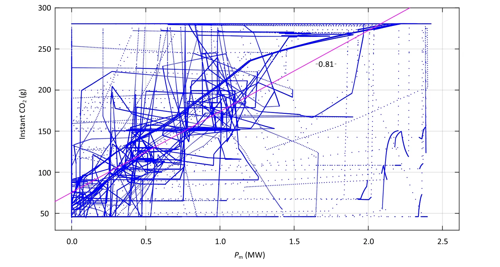
Fig. 9 Correlation of instant CO2 emission and traction mechanical power on diesel traction

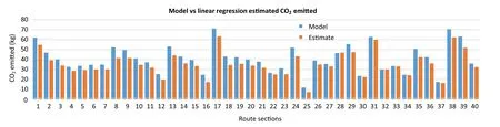
Fig. 10 Estimated and model total CO2 emitted in each section between Paddington and Swansea using linear regression

The route from Paddington to Swansea was also divided into 40 7.7-km sections,and Eq. (11)was used to estimate the mass of CO2from each of the sections. The high-fidelity model was then run over the same route and used to generate a more accurate CO2mass for each section. The results of these two methods are given in Fig. 10.It shows the difference between the total CO2estimated from Eq. (11)using Pm(t)for Paddington-Swansea and the total CO2obtained by running the high-fidelity train model over the same route. The maximum individual section difference was 38%, and the total CO2estimate from the linear regression model was within 10% of the high-fidelity model. This shows that while individual sections may differ,the linear regression model provides a fast model for estimation of CO2emissions and the rapid estimation of CO2emissions benefits of intermittent electrification. In this case,Pm(t)used as the input into the regression model for the Paddington-Swansea route was obtained by running the high-fidelity model. In the absence of a high-fidelity model, Pm(t) could be estimated by other means such as estimated speed and traction force profiles along a route.

5 Whole-life emissions modelling

The best way to decarbonise a railway is to electrify the entirety of the network whilst decarbonising the energy generation system. Discontinuous electrification in tandem with bi-mode rail vehicles should be a transitional solution on the path towards full electrification.If full electrification is not the final goal,then the fraction of electrification will depend on the considerations such as the carbon intensity of energy generation and the capital cost and embodied carbon dioxide in the electrification infrastructure.

This section will investigate the effects of including the carbon dioxide embodied in the electrification infrastructure (embodied emissions) in the overall lifetime CO2emissions(embodied emissions and operational emissions)of the given route. It will also investigate the effect of this on the cost per carbon dioxide saved for continuous and discontinuous electrification scenarios.

5.1 Net CO2 saving

Making baseline assumptions of the properties of the rail system (summarised in Table 4), it is possible to derive a comparison between discontinuous and continuous electrification and the net whole-life (embodied and operational) CO2saved through the two methods of electrification of the Newbury–Plymouth (currently unelectrified)section of the Paddington–Plymouth route. This analysis includes operational emissions (from running the trains)and embodied emissions (from erecting electrification infrastructure). The results of this analysis over a 50-year horizon are given in Fig. 11.

Figure 11 shows that discontinuous electrification provides higher net CO2savings per length of track electrified than continuous electrification. The ratio between their net CO2savings reaches a maximum of 2.3 at 10% electrification, and the difference between them reaches a maximum of 152 kt at 50% electrification. However, estimates for the embodied CO2in electrification systems vary, with some sources reporting this to be as low as 96 tCO2/doubletrack-km [30]. Several methods have been suggested for reducing the embodied carbon dioxide in electrification infrastructure,including reducing the weight of OLE masts and optimising the depth of foundation piles [29].

5.2 Cost per carbon saved

As discussed above, the cost of electrifying a dual-track route in the UK is approximately£2 M–5 M per kilometre[6], with costs increasing if the route includes tunnels or bridges [15]. In the near term, it may be reasonable to aim for the lowest cost-per-carbon-dioxide-saved method of electrification, as a cost-effective route to full electrification.

Using an average value of £3.5 M per double-track-km of electrification, it is possible to determine the cost (in pounds)per kg of CO2emissions prevented,and the results of this analysis are given in Fig. 12. This shows that discontinuous electrification is a cheaper cost-per-carbondioxide-saved method for steadily electrifying a given railway than the equivalent continuous electrification case.The peak difference between them is at 10%electrification,where discontinuous electrification costs 56% less per unitof CO2saved than continuous electrification of the same length of track.

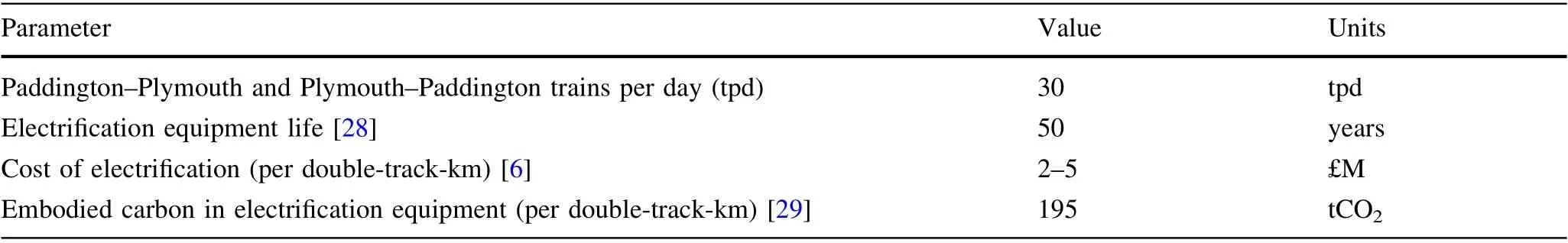
Table 4 Assumed values for carbon-cost accounting

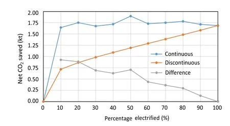
Fig. 12 Comparison of the total cost per CO2 saved between continuous and discontinuous electrification for the Newbury to Plymouth section of the Paddington-to-Plymouth route

However, this analysis comes with several caveats: the trade-off between continuous and discontinuous electrification is dependent on the embodied CO2in the electrification infrastructure, as described in Sect. 5.1. In addition,this is a first-order analysis using a fixed cost-per-kilometre for electrification. Electrification is a difficult process to cost accurately and depends upon many other factors including infrastructure such as bridges, tunnels, junctions and stations along the route. Furthermore, both electrification strategies (discontinuous and continuous) are different paths towards complete electrification, which is the only way to significantly reduce the CO2emissions of rail transport.

Also ignored for this analysis is the cost of the rolling stock.Bi-mode rolling stock is more complex as it has two power sources and is therefore more expensive than standard OLE-driven electric rolling stock. Additionally, this study has not considered the additional embodied emissions in the diesel engine-generator of a bi-mode rail vehicle.It is likely that including this would tip the balance towards full electrification at a lower percentage electrification than presented in this study.

6 Additional considerations for intermittent

electrification The analysis presented in this study has focussed on the carbon dioxide and cost cases for intermittent electrification as a transition pathway to a fully electrified rail network. There are a range of challenges associated with intermittent electrification that have not been considered here. For example, intermittent electrification—when compared to a continuous progressive electrification strategy—is likely to prove more logistically challenging, as the capital works equipment will have to be moved up and down the line several times, as different portions are electrified.

In addition, intermittent electrification poses difficulties when it comes to joining up two sections that have already been electrified. Each stretch of electrification will require its own substation to power the length of OLE. When two sections are subsequently joined (i.e. the section between them is electrified), there will be two substations feeding one section of OLE. This could be resolved by a small neutral insert (uncharged section of OLE) between the sections or by removing one of the substations. However,this implies that the capital cost of intermittent electrification could be higher due to increased number of substations when compared to a progressive electrification plan.

7 Conclusions

A high-fidelity model was used to determine the CO2emissions of a bi-mode rail vehicle operating under electric traction and diesel traction over the unelectrified section of a UK rail route.It was shown that CO2emissions for diesel running are higher than those for electric running,and that the CO2from electric traction depends on the carbon intensity of the electricity grid from which it is powered.

A near-optimal discontinuous electrification strategy was devised whereby the route from Newbury to Plymouth was split into 40 6.9-km sections and then sorted by CO2emissions, with the highest-emitting sections to be electrified first. When compared to continuous electrification starting from Newbury, this discontinuous electrification strategy saved more operational CO2per electrified length,to a maximum of 54% at 50% electrification. When normalised to grams of CO2per passenger-kilometre, discontinuous electrification has a maximum improvement of 12% over continuous electrification.

Linear regression was used to develop a simple model for CO2generation as a function of the traction power of the train. When this was used to analyse a second route(London Paddington to Swansea), the estimated CO2was within 10% of that produced by the high-fidelity model.This proves the viability of using regression models for faster emissions analysis of routes to determine the progression of any discontinuous electrification schemes than using the full high-fidelity model if an estimate of traction power is available.

Using existing values for infrastructure cost, lifetime and embodied CO2, this paper analysed the cost-per-carbon-dioxide-emissions performance and lifetime carbon dioxide saved per length of electrification for discontinuous and continuous electrification. It found that discontinuous electrification can save up to 2.3 times more CO2per distance electrified and can cost up to 56% less per reduction in lifetime emissions than continuous electrification. This concludes that discontinuous electrification can be an economic path to full electrification,and therefore maximal decarbonisation, of railway networks.

AcknowledgementsThe authors gratefully acknowledge the financial support of the EPSRC’s DTE Network + (EP/S032053/1)and the RSSB (COF-IPS-02).

Open AccessThis article is licensed under a Creative Commons Attribution 4.0 International License, which permits use, sharing,adaptation,distribution and reproduction in any medium or format,as long as you give appropriate credit to the original author(s) and the source,provide a link to the Creative Commons licence,and indicate if changes were made.The images or other third party material in this article are included in the article’s Creative Commons licence,unless indicated otherwise in a credit line to the material. If material is not included in the article’s Creative Commons licence and your intended use is not permitted by statutory regulation or exceeds the permitted use, you will need to obtain permission directly from the copyright holder. To view a copy of this licence, visit http://creativecommons.org/licenses/by/4.0/.