Variational quantum algorithms for trace norms and their applications

Sheng-Jie Li, Jin-Min Liang, Shu-Qian Shen and Ming Li

1 College of Science, China University of Petroleum, 266580 Qingdao, China

2 School of Mathematical Sciences,Capital Normal University, 100048 Beijing, China

Abstract The trace norm of matrices plays an important role in quantum information and quantum computing.How to quantify it in today’s noisy intermediate scale quantum(NISQ)devices is a crucial task for information processing.In this paper, we present three variational quantum algorithms on NISQ devices to estimate the trace norms corresponding to different situations.Compared with the previous methods, our means greatly reduce the requirement for quantum resources.Numerical experiments are provided to illustrate the effectiveness of our algorithms.

Keywords: quantum algorithm, trace norm, variational algorithm

1.Introduction

Quantum computing is a new ultrafast calculational model that follows the laws of quantum mechanics and regulates quantum information units for computing[1,2].A quantum computer can perform some computations with exponential speedup over any classical computer due to its intrinsic advantages.The famous quantum algorithms including Shor’s factoring algorithm [3],Grover’s search algorithm[4]and HHL algorithm[5]for linear equations most require a universal fault-tolerant quantum computer with millions of qubits [1].Most of these algorithms have deep circuit depth, and the coherence between quantum states will gradually lost due to the undesired environmental noise.Thus, the appearance of such experimental device may take many years of research.Noisy intermediate scale quantum(NISQ)technology[6,7]adopting 50–100 qubits is believed to be an high-performance alternative product.It will be available in the near future.Hence, one of the current researches focuses on the algorithms that can efficiently work on the NISQ devices.

The class of variational quantum algorithms (VQAs)[8, 9],which is a kind of hybrid quantum–classical algorithms, is considered to be well-suited in the NISQ period.By utilizing the classical computers and NISQ devices simultaneously, VQAs solve problems that are intractable on classical computers.To be specific,VQAs adopt the classical computers to find the optimal parameters of the objective function,and quantum devices mainly compute the values of function by training the neural networks and performing measurements.In recent years, a variety VQAs have been proposed such as variational eigenvalue solver[10–14], variational quantum singular value decomposition[15,16],variational quantum diagonalization[17,18],quantum approximate optimization algorithms [19], variational ansatzbased quantum simulation [20], and quantum linear equations solver [21, 22]; see, e.g.[8, 9] for comprehensive surveys.In addition, quantum simulation is also another important application of near-term quantum computing; see, e.g.[23–27].

Trace norms have been widely used in the field of quantum information and quantum computing.As we all know, the detection and quantification of entanglement is a fundamental issue in quantum information.Some separable criteria including CCNR [28], correlation matrix criteria [29] are based on trace norms.They can also be used to quantify entanglement[30]and non-locality [31].Meanwhile, the trace distance based on trace norms yields a natural metric on the state space, and gives a measure of the distinguish ability between two quantum states[2].In addition,a lot of quantum machine learning algorithms such as quantum anomaly detection [32], dimensionality reduction and classification [33] are also based on the trace norms.Generally speaking, the estimation of trace norms on classical computers needs to calculate all singular values [34].However, the calculation of singular values of large-scale matrices is still a tricky task for classical computers, which consumes tremendous resources especially when the matrix dimension reaches the exponential order.Thus, how to evaluate the trace norms efficiently on quantum devices is an essential task.

VQAs for estimating the trace norms and trace distances have been presented in [35].It variationally estimates trace norms by adding an ancillary system and performing the unitary evolution on the whole system.From the perspective of near-term implementation, it will increase operation difficulty.

The aim of this paper is to design novel VQAs for trace norms, which can be applied to the estimation of trace distance, detection and quantification of quantum entanglement.The cost of algorithms are less than the corresponding ones in[35].Finally,we simulate our algorithms to estimate the trace norms of two qubit matrix and obtain the desired result.

The organization of the paper is as follows.In section 2,we briefly review the trace norms and introduce a proposition which is beneficial to apply optimization methods on the loss function.Then we present our VQAs for estimating trace norms which we call them the quantum variational trace norm(QVTN)algorithms.Some applications including trace distance estimation and quantification of quantum entanglement are presented in section 3.Numerical experimental simulations are reported in section 4.Then we make a summary in section 5.

2.Results

2.1.Theoretical basis for QVTN alogrithms

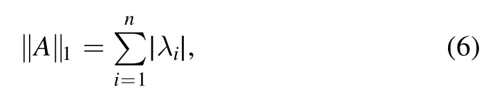
Let A be an operator acting on a Hilbert spaceH.Then we denote by ‖A‖1the trace norm of A, i.e.the sum of all singular values of A.From [2], we can get

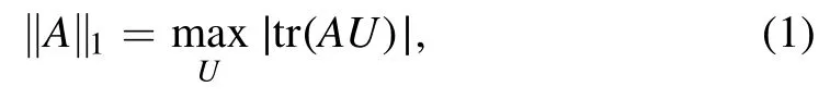
wheretr denotes the trace of matrix, and the maximization ranges over all unitary operators acting onH.Obviously, the equality(1)cannot be directly applied to design VQAs,since some optimization methods cannot be used for the absolute value function.The following simple proposition gives an alternative to (1), and then VQAs can be easily constructed.

Proposition 1.Let A be any operator acting on the Hilbert spaceH.Then

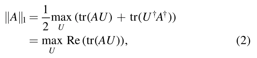
where the optimization is over all unitary operators acting on systemH, and† denotes the conjugate transpose of matrix.

Proof.On the one hand, by (1),

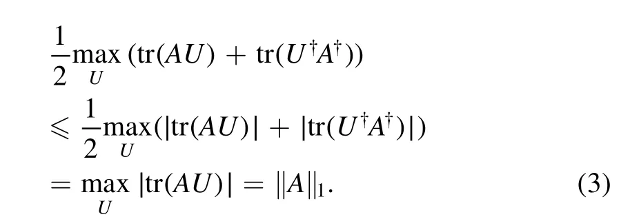
On the other hand,by(1)there must exist a unitary operator V and a real number θ such that

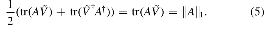
This completes the proof. □

For any Hermitian operator A, it is easy to get

where λi, i=1, 2, …, n, are eigenvalues of A.If A is not Hermitian, we can define the operator

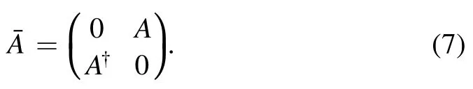
From [5],is Hermitian, andThus, in this section,the VQAs are only designed for Hermitian operators.

Proposition 1 gives us a favorable variational form.According to this form, in the next subsections, we will present VQAs (QVTN) to estimate the trace norms of the Hermitian operator H.

2.2.The QVTN algorithm based on state decomposition

Assume that H acting on the Hilbert spaceH is Hermitian,then H can always be decomposed [2, 35] as

where ri,i=1,2,…,d,are real numbers,and ρi,i=1,2,…,d, are density matrices.In fact, any Hermitian matrix can easily be decomposed into the above form; see, e.g.equation (14) in algorithm 2.Meanwhile, the calculation of generalized trace distance in section 3 also uses the decomposition as a special case of equation (8).Based on (8), the following VQA gives the estimation of the trace norm of H.

Algorithm 1.The QVTN algorithm based on state decomposition

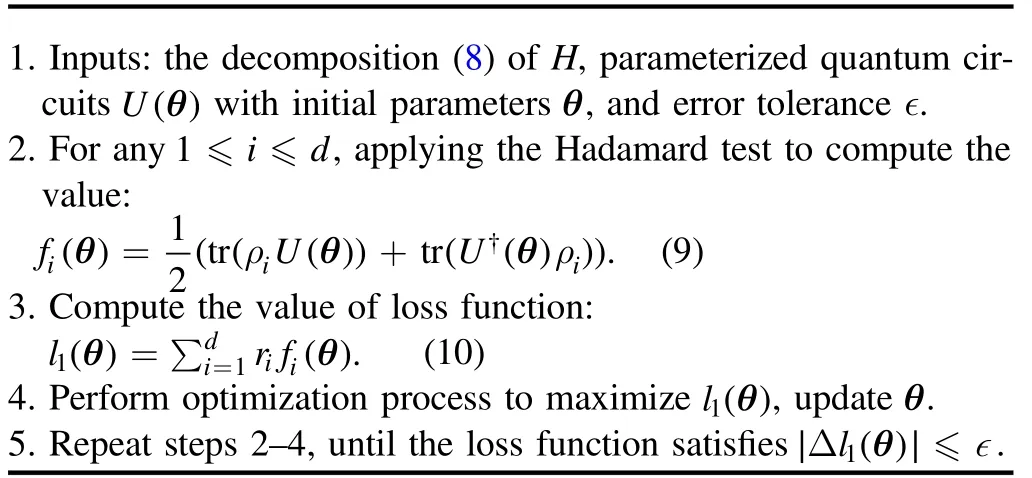
1.Inputs: the decomposition (8) of H, parameterized quantum circuits U( θ)with initial parameters θ, and error tolerance ∈.2.For any ≤ i≤ d 1 , applying the Hadamard test to compute the value:() ( ( ()) ( ()))†θ=θ θρ ρ+f U U 1 2 tr tr .i i i (9)3.Compute the value of loss function:() ()θ θ= ∑=l r f .i d i i 1 1(10)4.Perform optimization process to maximize l( θ)1 , update θ.5.Repeat steps 2–4, until the loss function satisfies∣ Δ( θ)∣≤∈l1 .

As in [16, algorithm 1], the parameterized quantum circuits is composed by single qubit rotations and two qubit CNOT gates and here the parameterθ= (θ1,θ2, … ,θ m)t,where t represents the transpose of matrix.Figure 1 is a schematic diagram of the circuits.Specifically, the parameterized circuits

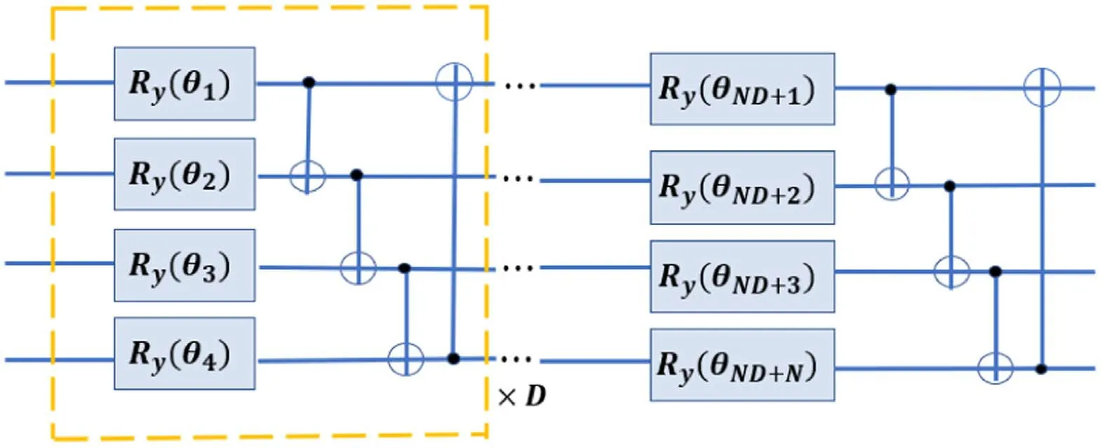
Figure 1.The parameterized quantum circuit for U(θ).The parameters are trained to optimize the loss functions.Here D denotes the circuit depth and N represents the qubit numbers.

For j=1, 2, …, m, we consider

where Hjis tensor product of Pauli matrices.

Proposition 2.The loss functionl1(θ)and the gradient of it can be estimated on near-term quantum devices.

Proof.Our loss function can be efficiently computed by the Hadamard test[36].The schematic diagram is shown in figure 3.We briefly summarize the key points of Hadamard test here.

In the step 2 of algorithm 1,by adding an ancillary qubit,Re ( tr (ρU))for any state ρ and unitary U can be computed by quantum Hadamard test.As in figure 3, after the application of the circuit before measurement, the initial statesδin= ∣0 〉 〈 0∣⊗ρbecomes

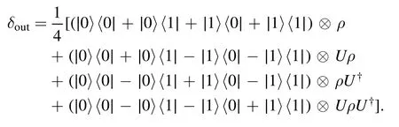
Measuring the ancillary state with the Pauli operatorσzyields the expectation value

Thus the loss functionl1(θ)can be efficiently calculated in near-term devices by the Hadamard test.

In addition, according to the specific calculation process in appendix, we get a fact that the derivatives of the loss functionl1(θ)are given by several terms which can be estimated by rotating the parameters of the Hadamard test circuits in figure 3.Hence, the gradient of loss functionl1(θ)can be estimated on near-term quantum devices. □

If the decomposition of H (8) is not available, we can choose a parameter α to construct the following two states:

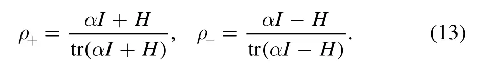
For example, α can be chosen to be ∑i|hii| with hiibeing the diagonal element of H.For this case, a simplified form of algorithm 1 is given by algorithm 2.

Algorithm 2.The QVTN algorithm based on QRAM

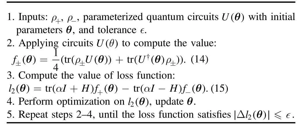
1.Inputs:ρ ρ+, - , parameterized quantum circuits U( θ)with initial parameters θ, and tolerance ∈.2.Applying circuits U( θ)to compute the value:() ( ( ()) ( ()))†θ=θ θρ ρ+±±±f U U 1 4 tr tr .(14)3.Compute the value of loss function:() () () () ()θ θ α= + - -+-l αI H f I H fθ tr tr .2(15)4.Perform optimization on l( θ)2 , update θ.5.Repeat steps 2–4, until the loss function satisfies∣Δ ( θ)∣≤∈l2 .

In the step 2 of algorithm 2,we can use swap test[37]to compute the trace of the product of a density matrix and a unitary matrix.Given a general quantum state ρ, it can be expressed as a linear combinationin the computation basis.The vector representation of ρ can be written as

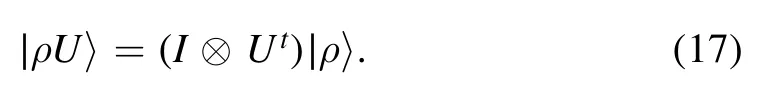
Finally,

can be efficiently estimated via the simple swap test.

However, the QRAM approach requires great amount of qubits to convert classical data into corresponding quantum states[40],making it not suitable in the current NISQ devices.Here we give alternative methods to efficiently obtain the state|I〉.Figure 2 shows the corresponding quantum circuit to implement |I〉, consisting of the Hadamard gate H, Pauli operator σzand CNOT gates.To our knowledge, there is no effective method to prepare |ρ〉 except QRAM.Thus, for the preparation of |ρ〉, it is worth studying new methods that are suited for the NISQ devices in the future.

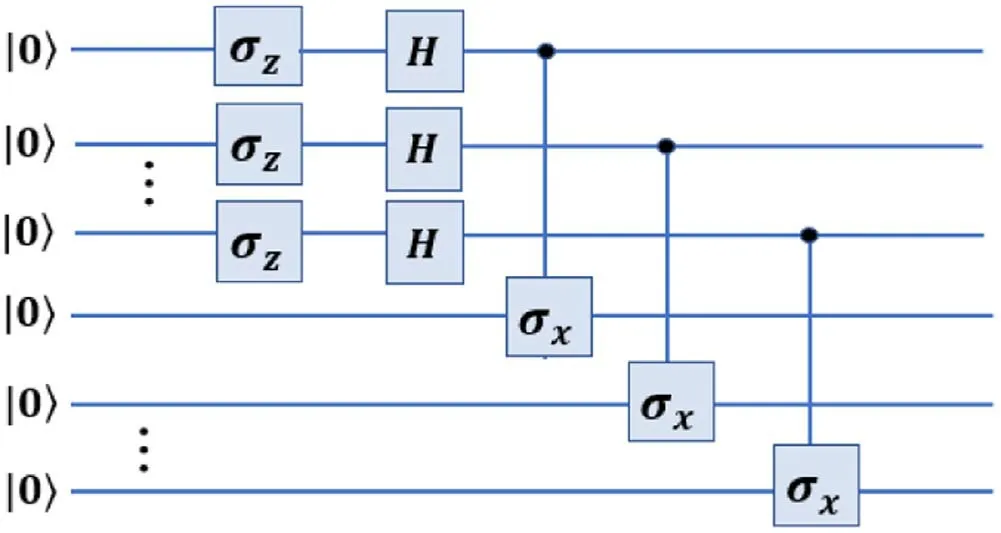
Figure 2.The preparation for state |I〉.

2.3.The QVTN algorithm based on unitary decomposition

Assume that the Hermitian operator H acting on the Hilbert spaceH can be written as

where ki,i=1,2,…,n,are real numbers and Ui,i=1,2,…,n,are unitary matrices.This assumption is often employed in many physical systems such as molecules or the Fermi–Hubbard model [13, 16, 41].Based on (19), the following VQA gives the estimation of the trace norm of H.

Algorithm 3.The QVTN algorithm based on unitary decomposition

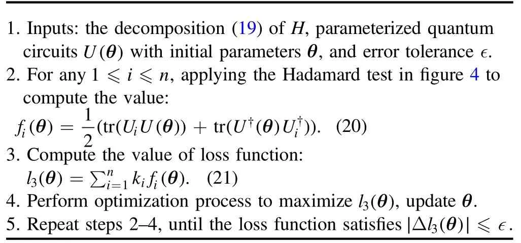
1.Inputs: the decomposition (19) of H, parameterized quantum circuits U( θ)with initial parameters θ, and error tolerance ∈.2.For any ≤ i≤ n 1 , applying the Hadamard test in figure 4 to compute the value:() ( ( ()) ( ()))† †θ=θ θ+f U U U U 1 2 tr tr .i i i (20)3.Compute the value of loss function:() ()θ θ= ∑=l k f .in i i 3 1 (21)4.Perform optimization process to maximize l( θ)3 , update θ.5.Repeat steps 2–4, until the loss function satisfies∣ Δ ( θ)∣≤∈l3 .

It is obvious that when we replace the state ρ with identity matrix I in figure 3, tr(UiU)for any unitary Uiand U can be computed by the Hadamard test.We draw a simple diagram in figure 4.Thus,the loss function l3(θ)in algorithm 3 can be efficiently calculated in near-term quantum devices.In addition,the optimization of functions l1(θ),l2(θ)and l3(θ)will be discussed in section 4.

Recently, Wang et al [16] provide a VQA for determining the largest T singular values of a given n×n matrix M,the related loss function L(α,β)is the linear combination of Re〈ψj∣U†(α)MV(β)∣ψj〉with weight qj, j=1, 2, …, T.Hereare computational basis and U(α), V(β) are unitary circuits.We notice that this method can also give an estimation of the trace norm by calculating all singular values when T=n.Compared with it,our algorithms directly obtain an estimation of the trace norm through training parameters instead of requiring the specific information of all singular values.Thus, our methods greatly reduce the demands of quantum resources and circuits complexity.In addition, our loss functions only contain one parameter vector which are more conducive for us to find the global optimum.

The paper [35] also have proposed a VQA for trace norms of Hermite matrix.They evaluated the trace norms due to the following formula

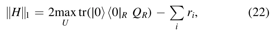
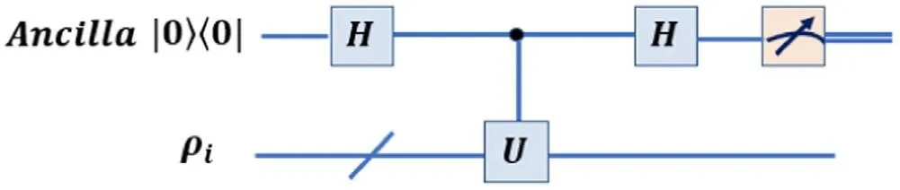
Figure 3.The Hadamard test for estimating tr( ρU).

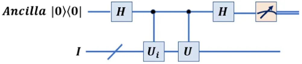
Figure 4.The Hadamard test for estimating tr(Ui U).

whereQR=trAQ AR, QAR=U(H ⊗|r〉〈r|R)U†, |r〉 is an ancillary qubit in system R,and the optimization is over all unitary matrices on composite system AR.Compared with it, our methods have the following advantages.On the one hand,our algorithms do not need purification of the quantum state which may be hard to implement in near-term quantum circuits.On the other hand, we only use an ancillary qubit to compute the value of loss function instead of participating in the unitary evolution process of the whole system.Thus, our main variational processes are only local unitary evolution which greatly reduces the difficulty of operation and resource requirements.

3.Applications

3.1.Estimation of generalized trace distances

The generalized distance [42, 43] is a measure of non-Markovianity for an open system dynamics which has significant effect in digital geometry.The generalized trace distance between two states ρ and σ acting on the Hilbert spaceH is defined as

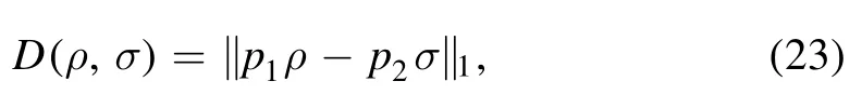
where p1and p2are real numbers.Therefore, we design the following functions from algorithm 1 to estimate the generalized trace distances.Let

then we choose

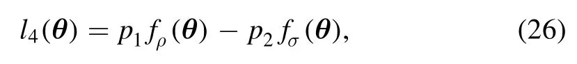
as our loss function which is the linear combination of fρ(θ)and fσ(θ).

It is of great significance because the trace distance qualifies how different the two quantum states are.

3.2.Variational algorithms for recognizing and quantifying entanglement

Our VQAs can also be used for recognizing and quantifying entanglement.In this section, we review the bipartite entanglement and use QVTN algorithms for recognizing and quantifying entanglement.

A bipartite state ρ is said to be separable[44,45]if it can be written as

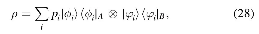
where 0 ＜pi≤1, ∑ipi=1, and{∣φi〉}iand{∣φi〉}iare pure states on subsystem A and B, respectively.Consequently, a bipartite state ρ is entangled if it cannot be decomposed into the above form.

The realignment criterion in [46] says that a bipartite quantum state ρABinCk1⊗Ck2is separable, then

where R(ρAB)is the realignment matrix of ρAB.Thus we can judge that a state ρABis entangled by calculating the trace norm ‖R(ρAB)‖1according to our QVTN algorithms.The QVTN algorithms are also useful in permutation criterion[47]and correlation matrix criteria[29]by estimating trace norms.

As we all know the logarithmic negativity [45, 48] of a quantum state is a good entanglement measure which has wide applications in quantum information.The logarithmic negativity of a bipartite state ρABis defined as

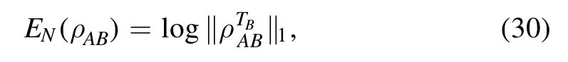
where TBis the partial transpose with subsystem B.So the logarithmic negativity can be efficiently estimated by our QVTN algorithms.

4.Numerical experiments

4.1.Optimization of the loss function

In this section, we discuss the optimization of loss functions li(θ)for i=1,2,3,4.There are many optimization algorithms ranging from gradient-free methods to gradient-based methods.Here we choose gradient descent (GD) [49] algorithm which can be used for first-order gradient-based optimization of loss functions.

GD algorithm is a common method to solve unconstrained optimization problems, and has a wide range of applications in optimization, statistics, and machine learning.This method is generally used to find the minimum value of the objective functions.We need to select the initial parametersproperly, and then move to the next point according to the gradient direction of the objective function.The iterative formula is as follows:

the parameter γ is a positive learning rate which determines the step length of each iteration and hereSee the appendix for the specific process of calculating the gradient of li(θ) for i=1, 2, 3, 4.

4.2.Numerical experiments

In this section, we apply our algorithms 1 and 3 to estimat e the trace norm of two qubit Hermite matrix.We utilize a hardware efficient ansatz in the simulation including parameterized Ryand Rzoperations and CNOT gates.Consider the following matrix

where σxand σzare the Pauli matrices.Our experiments apply a quantum circuit with L=2 layers with initial state|ψin〉=|0〉⊗|0〉.All numerical simulations and optimization are prepared via Paddle Quantum [50] on the PaddlePaddle Deep Learning Platform [51].The figure 5 plots the trace norm of matrix M via iterations.Our experiment values are presented with purple dashed line compared with theoretical result with blue points.The learning rate we set is LR=0.1.As shown in figure 5, we can see that the loss function has reached global optimum corresponding to the theoretical result.Thus, we can find the the trace norm of matrix M and obtain the associated parameter θopt.The quantum parameterized circuit after training is shown in figure 6.

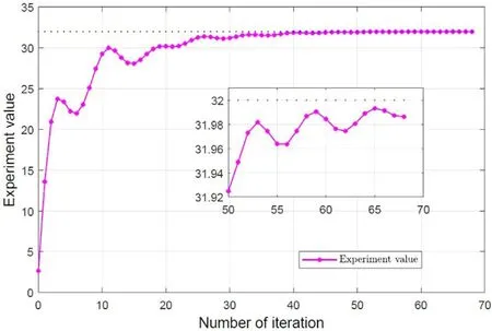
Figure 5.The trace norm of matrix M learned by our QVTN algorithms.

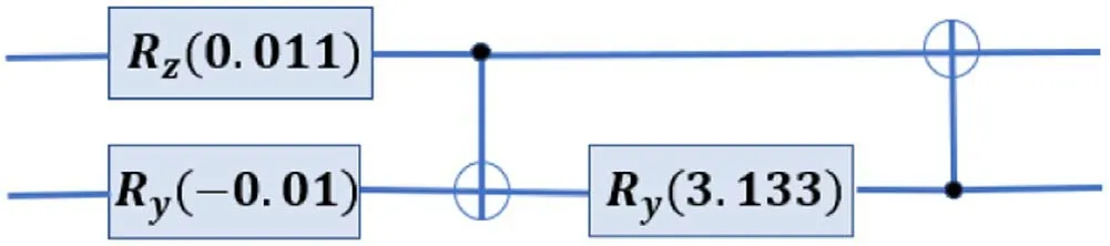
Figure 6.The quantum parameterized circuit after training used in numerical simulations.

5.Conclusions

In conclusion, we have presented three VQAs for estimating trace norms.The algorithms 1 and 2 are based on state decomposition, and algorithm 3 is based on unitary decomposition.The advantages of our algorithms are as follows.Firstly, our algorithms do not need Hamiltonian simulation[52], phase estimation [2] and amplitude amplification [53],showing efficient availability in NISQ era.Secondly, our method directly estimate the value of the trace norms rather than their bounds.Thirdly,our main variational processes are local unitary evolution which greatly reduces the cost.

Our algorithms have a wide range of applications in quantum information.A direct application is to calculate the trace distance that can be applied to quantify the distinction between two quantum states.Our algorithms may have further applications in quantifying the security of quantum cryptography protocols[54]and Bell non-locality[55],which have significant effects in entanglement, coherence and other quantum resources [56–58].

Acknowledgments

The authors thank the referees and the editor for their invaluable comments.

Appendix.Optimization of the loss functions

In this section, we present the detailed calculation process on the gradients of the loss functions li(θ) for i=1, 2, 3, 4.

Consider the parameterized circuits

where the second equality is due to the following property

Therefore

whereθ+j= (θ1,… ,θj+π,… ,θm)t.

Similarly, we have

We know, in algorithm 1, the loss function

where, for 1 ≤i ≤d,

So

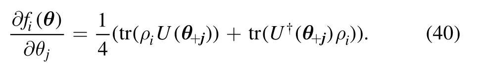
Hence,

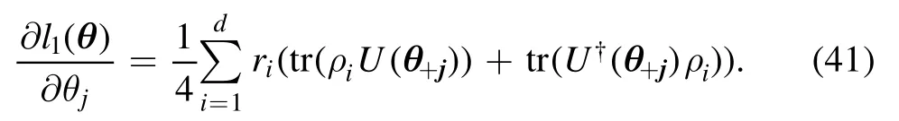
We can perform the same process to compute the gradient of l2(θ), l3(θ) and l4(θ).