Deep learning neural networks for the thirdorder nonlinear Schrödinger equation:bright solitons, breathers, and rogue waves

Zijian Zhou and Zhenya Yan,*

1 Key Laboratory of Mathematics Mechanization,Academy of Mathematics and Systems Science,Chinese Academy of Sciences, Beijing 100190, China

2 School of Mathematical Sciences, University of Chinese Academy of Sciences, Beijing 100049, China

Abstract The dimensionless third-order nonlinear Schrödinger equation (alias the Hirota equation) is investigated via deep leaning neural networks.In this paper,we use the physics-informed neural networks(PINNs)deep learning method to explore the data-driven solutions(e.g.bright soliton,breather, and rogue waves) of the Hirota equation when the two types of the unperturbated and perturbated(a 2%noise)training data are considered.Moreover,we use the PINNs deep learning to study the data-driven discovery of parameters appearing in the Hirota equation with the aid of bright solitons.

Keywords:third-order nonlinear Schrödinger equation,deep learning,data-driven solitons,datadriven parameter discovery

1.Introduction

As a fundamental and prototypical physical model, the nonlinear Schrödinger (NLS) equation is

where q = q(x, t) denotes the complex field, and the subscripts stand for the partial derivatives with respect to the variables,σ = 1 and σ = -1 corresponds to the focusing and defocusing interactions, respectively.Equation (1) can be used to describe the wave propagation in many fields of Kerr nonlinear and dispersion media such as plasmas physics,deep ocean, nonlinear optics, Bose–Einstein condensate, and even finance (see, e.g.[1–8] and references therein).When the ultra-short laser pulse (e.g.100 fs [7]) propagation were considered, the study of the higher-order dispersive and nonlinear effects is of important significance, such as thirdorder dispersion, self-frequency shift, and self-steepening arising from the stimulated Raman scattering [9–11].The third-order NLS equation (alias the Hirota equation [12]) is also a fundamental physical model.The Hirota equation and its extensions can also be used to describe the strongly dispersive ion-acoustic wave in plasma [13] and the broaderbanded waves on deep ocean[14,15].The Hirota equation is completely integrable, and can be solved via the bi-linear method [12], inverse scattering transform [16, 17], and Darboux transform (see, e.g.[18–22]), and etc.Recently, we numerically studied the spectral signatures of the spatial Lax pair with distinct potentials (e.g.bright solitons, breathers,and rogue waves) of the Hirota equation [23].

Up to now, artificial intelligence and machine learning have been widely used to powerfully deal with big data, and play a more and more important role in the various fields,such as language translation, computer vision, speech recognition, and so on [24, 25].More recently, the deep neural networks were presented to study the data-driven solutions and parameter discovery of nonlinear physical models [26–36].Particularly, the physics-informed neural networks(PINNs)technique[28,32]were developed to study nonlinear partial differential equations.In this paper, we would like to extend the PINNs deep learning method to investigate the data-driven solutions and parameter discovery for the focusing third-order NLS equation (alias the Hirota equation) with initial-boundary value conditions

where q = q(x, t) is a complex envelope field, α and β are real constants for the second- and third-order dispersion coefficients, respectively.For β = 0, the Hirota equation (2)becomes a NLS equation, whereas α = 0, the Hirota equation (2) reduces to the complex modified KdV equation [12].

2.The PINN scheme for the data-driven solutions

2.1.The PINNs scheme

In this section, we would like to simply introduce the PINN deep learning method [32] for the data-driven solutions.The main idea of the PINN deep learning method is to use a deep neural network to fit the solutions of equation (2).Letq(x,t) =u(x,t) +iv(x,t)withu(x,t) ,v(x,t)being its real and imaginary parts,respectively.The complex-valued PINNF(x,t) =Fu(x,t) +iFv(x,t) withFu(x,t) ,Fv(x,t) being its real and imaginary parts, respectively are written as

and proceeded by approximating q(x,t)by a complex-valued deep neural network.In the PINN scheme, the complexvalued neural networkq(x,t) =(u(x,t) ,v(x,t)) can be written as

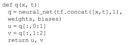
Based on the defined q(x, t), the PINN F(x, t) can be taken as

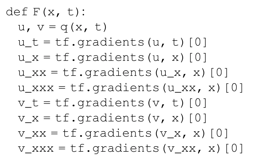
The shared parameters, weights and biases, between the neural network=u(x,t) +iv(x,t) andF(x,t)=Fu(x,t) +iFv(x,t) can be learned by minimizing the whole training loss (TL), that is, the sum of theL2-norm TLs of the initial data (TLI), boundary data (TLB), and the whole equation F(x, t) (TLS)

where the mean squared (i.e.L2-norm) errors are chosen for them in the forms

We would like to discuss some data-driven solutions of equation (2) by the deep learning method.Here we choose a 5-layer deep neural network with 40 neurons per layer and a hyperbolic tangent activation functiontanh(·)

to approximate the learning solutions, whereAj=anddenote the output and bias column vectors of the jth layer, respectively,stands for the weight matrix of the jth layer,A0= (x,t)T,AM+1=(u,v)T.The real and imaginary parts, u(x, t) and v(x, t), of approximated solution=u(x,t) +iv(x,t) are represented by the two outputs of one neural network (see figure 1 for the PINN scheme).In the following, we consider some fundamental solutions (e.g.bright soliton, breather, and rogue wave solutions) of equation (2) by using the PINNs deep leaning scheme.For the caseαβ≠0 in equation (2),without loss of generality, we can take α = 1, β = 0.01.

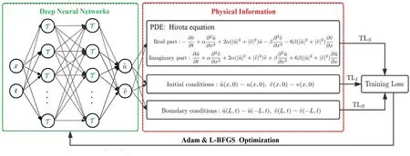
Figure 1.The PINN scheme solving the Hirota equation(2)with the initial and boundary conditions,where the activation function T= tanh(·).

2.2.The data-driven bright soliton

The first example we would like to consider is the fundamental bright soliton of equation (2) [9, 12]

where the third-order dispersion coefficient β stands for the wave velocity, and the sign of β represents the direction of wave propagation [right-going (left-going) travelling wave bright soliton for β ＞0 (β ＜0)].

We here choose L = 10,t0= 0,T = 5,and will consider this problem by choosing two distinct kinds of initial sample points:In the first case,we will choose the NI= 100 random sample points from the initial dataqbs(x,t=0) withx∈ [- 10, 10].But in the second case, we only choose NI= 5 sample points from the initial dataqbs(x,t=0) with 5 equidistant and symmetric pointsx∈ {- 5, -2.5,0, 2.5, 5}.In the both cases, we use the same NB=200 periodic boundary random sample points and NS=10 000 random sample points in the solution region{(x,t,qbs(x,t))∣(x,t) ∈ [- 10, 10] ×[0 , 5]}.It is worth mentioning that the NS= 10 000 sample points are obtained via the Latin Hypercube Sampling strategy [37].

We emulate the first case of initial data by using 10 000 steps Adam and 10 000 steps L-BFGS optimizations such that figures 2(a1)–(a3)and(b1)–(b3)illustrate the learning results starting from the unperturbated and perturbated (2% noise)training data, respectively.The relative L2- norm errors of q(x, t), u(x, t) and v(x, t), respectively, are 9.3183 ×10-3, 5.3270 × 10-2, 3.8502 × 10-2in figures 2(a1)–(a2),and 7.0707 × 10-3, 2.4057 × 10-2, 1.6464 × 10-2in figures 2(b1)–(a2).Similarly, we use the 20 000 steps Adam and 50 000 steps L-BFGS optimizations for the second case of initial data such that figures 2(c1)–(c3) and (d1)–(b3)illustrate the learning results starting from the unperturbated and perturbated training data, respectively.The relative L2-norm errors of q(x, t), u(x, t) and v(x, t), respectively,are 1.8822 × 10-2, 4.9227 × 10-2, 4.0917 × 10-2in figures 2(c1)–(c2), and 2.5427 × 10-2, 3.4825 × 10-2,2.5983 × 10-2in figures 2(d1)–(d2).Notice that those total learning times are(a)717s,(b)741s,(c)1255s,and(d)1334s,respectively,by using a Lenovo notebook with a 2.6 GHz sixcores i7 processor and a RTX2060 graphics processor.

Remark.In each step of the L-BFGS optimization, the program is stop at

where the loss(n) represents the value of loss function in the nth step L-BFGS optimization, and1.0 ×np.finfo (f loat).eps represent Machine Epsilon.When the relative error between loss(n)andloss(n-1)less than Machine Epsilon,procedure would be stop.This is why the computation times are different for each test by using the same step optimization.

2.3.The data-driven AKM breather solution

The second example we would like to study is the AKM breather (spatio-temporal periodic pattern) of equation (2)[18]

whereξ=x- 2β[2 +cos (2c)t],ω=2 sin (2c),p=2 sin(c),and c is a real constant.The wave velocity and wavenumber of this periodic wave are2β(2 + cos (2c)) and p, respectively.This AKM breather differs from the Akhmediev breather (spatial periodic pattern) of the NLS equation because equation(2)contains the third-order coefficient β.In this example, we assume β = 0.01 again.Whent→∞,∣qakm(x,t)∣2→1.Ifβ→0, we haveξ→x, and then AKM breather almost becomes the Akhmediev breather.

We here choose L = 10 andt∈ [-3, 3],and choose the NI= 100 random sample points from the initial dataqakm(x,t=0), NB= 200 random sample points from the periodic boundary data, and NS= 10 000 random sample points in the solution region (x,t) ∈ [- 1 0, 10] × [- 3, 3].We use the 20 000 Adam and 50 000 L-BFGS optimizations to learn the solutions from the unperturbated and perturbated(a 2% noise) initial data.As a result, figures 3 (a1)–(a3) and(b1)–(b3)exhibit the leaning results for the unperturbated and perturbated (a 2% noise) cases, respectively.The relative L2-norm errors of q(x, t), u(x, t) and v(x, t), respectively, are(a) 1.1011 × 10-2, 3.5650 × 10-2, 5.0245 × 10-2, (b)1.3458 × 10-2,5.1326 × 10-2,7.0242 × 10-2.The learning times are 2268 s and 1848 s, respectively.

2.4.The data-driven rogue wave solution

The third example is a fundamental rogue wave solution of equation (2), which can be generated when one takesc→0 in the AKM breather (9) in the form [19]

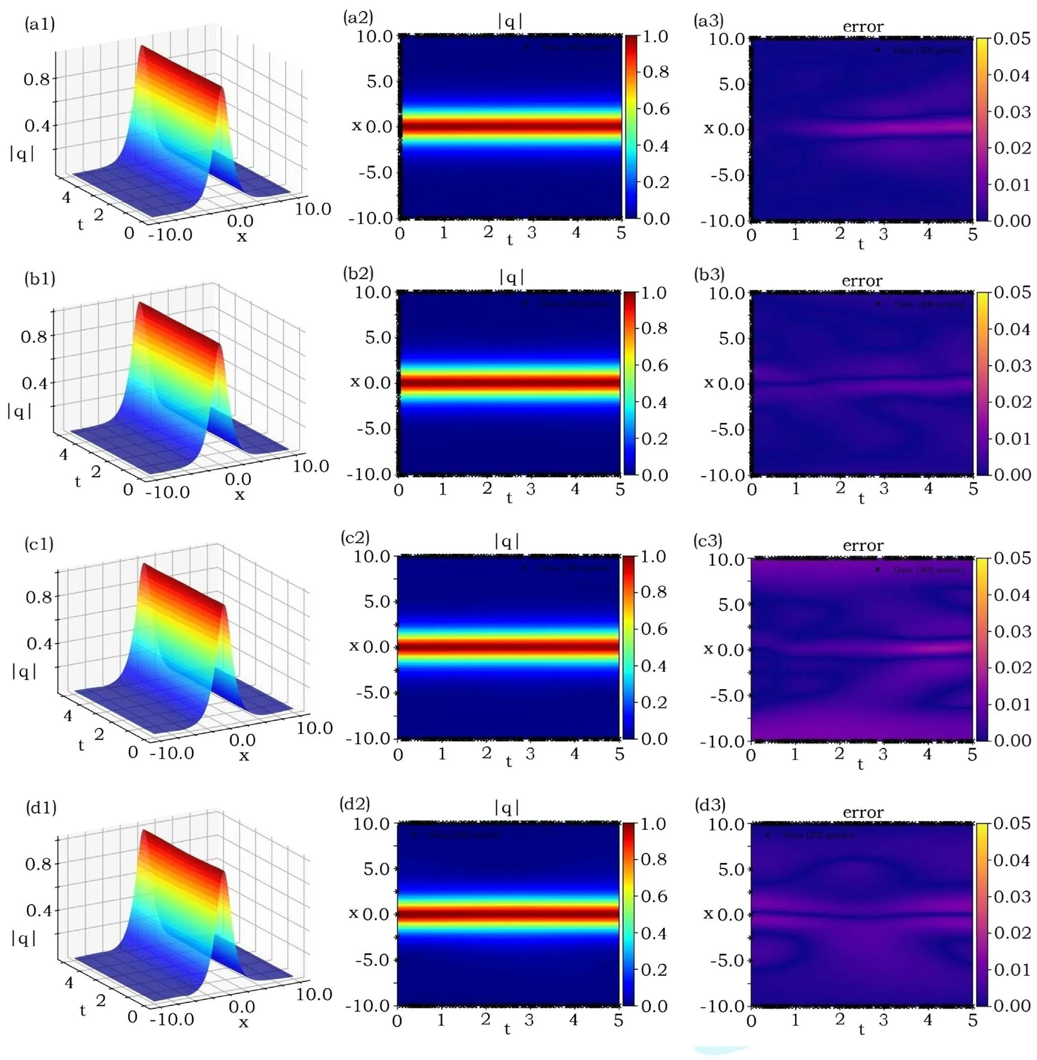
Figure 2.Data-driven bright soliton of the Hirota equation(2):(a1),(a2)and(b1),(b2)the learning solutions arising from the unpeturbated and perturbated(2%)training data related to the first case of initial data,respectively;(c1),(c2)and(d1),(d2)the learning solutions arising from the unpeturbated and perturbated(2%)training data related to the first case of initial data,respectively;(a3),(b3),(c3),(d3)the absolute values of the errors between the modules of exact and learning solutions.The relative L2- norm errors of q(x, t), u(x, t) and v(x, t),respectively, are (a1)–(a3) 9.3183 × 10-3, 5.3270 × 10-2, 3.8502 × 10-2, (b1)–(b3) 7.0707 × 10-3, 2.4057 × 10-2, 1.6464 × 10-2,(c1)–(c3) 1.8822 × 10-2, 4.9227 × 10-2, 4.0917 × 10-2, (d1)–(d3) 2.5427 × 10-2, 3.4825 × 10-2, 2.5983 × 10-2.

Figure 3.Learning breathers related to the AKM breather(9)of the Hirota equation(2).(a1)–(a3)The unperturbated case,(b1)–(b3)the 2%perturbated case.The relative L2- norm errors of q(x, t), u(x, t) and v(x, t), respectively, are (a1)–(a3) 1.1011 × 10-2, 3.5650 × 10-2,5.0245 × 10-2, (b1)–(b3) 1.3458 × 10-2, 5.1326 × 10-2, 7.0242 × 10-2.

As ∣x∣ ,∣t∣ →∞,∣qrw∣ →1, and maxx,t∣qrw∣ =3.

We here choose L = 2.5 andt∈ [- 0.5, 0.5], and considerqrw(x,t= -0.5) as the initial condition.We still choose NI= 100 random sample points from the initial dataqrw(x,t= -0.5), NB= 200 random sample points from the periodic boundary data, and NS= 10 000 random sample points in the solution region (x,t) ∈ [- 2 .5, 2.5]×[- 0.5, 0.5].We use the 20 000 steps Adam and 50 000 steps L-BFGS optimizations to learn the rogue wave solutions from the unperturbated and perturbated (a 2% noise) initial data,respectively.As a result, figures 4(a1)–(a3) and (b1)–(b3)exhibit the leaning results for the unperturbated and perturbated (a 2% noise) cases, respectively.The relative L2- norm errors of q(x, t), u(x, t) and v(x, t), respectively, are(a) 6.7597 × 10-3, 8.8414 × 10-3, 1.6590 × 10-2, (b)3.9537 × 10-3, 5.8719 × 10-3, 9.0493 × 10-3.The learning times are 1524 s and 1414 s, respectively.

3.The PINNs scheme for the data-driven parameter discovery

In this section, we apply the PINNs deep learning method to study the data-driven parameter discovery of the Hirota equation (2).In the following, we use the deep learning method to identify the parameters α and β in the Hirota equation (2).Moreover, we also use this method to identify the parameters of the high-order terms of equation (2).

3.1.The data-driven parameter discovery for α and β

Here we would like to use the PINNs deep learning method to identify the coefficients α, β of second- and third-order dispersive terms in the Hirota equation

where α, β are the unknown real-valued parameters.

Letq(x,t) =u(x,t) +iv(x,t) withu(x,t) ,v(x,t)being its real and imaginary parts, respectively, and the PINNsF(x,t) =Fu(x,t) +iFv(x,t) withFu(x,t) ,Fv(x,t)being its real and imaginary parts, respectively, be

Then the deep neural network is used to learn{u(x,t) ,v(x,t)} and parameters (α, β) by minimizing the mean squared error loss

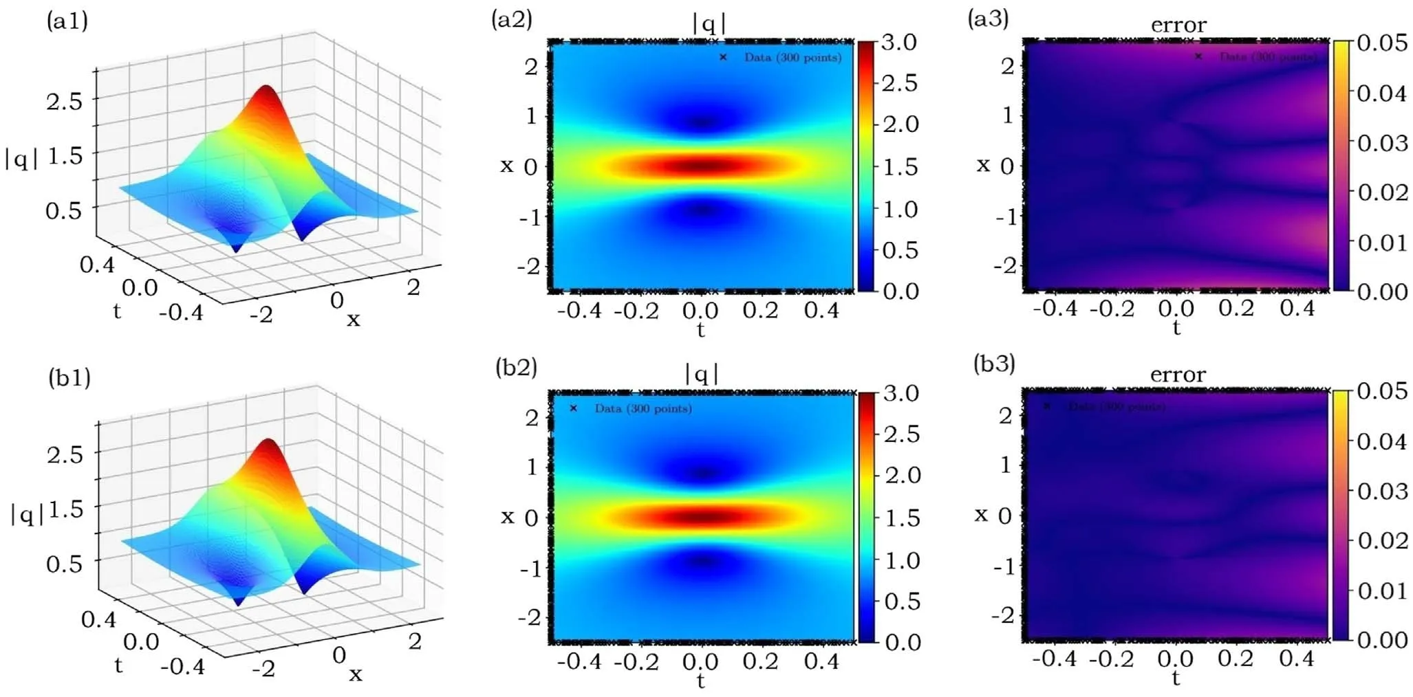
Figure 4.Learning rogue wave solution related to equation(10)of the Hirota equation(2).(a1)–(a3) The unperturbated case,(b1)–(b3)the 2% perturbated case.The relative L2- norm errors of q(x, t), u(x, t) and v(x, t), respectively, are (a1)–(a3) 6.7597 × 10-3, 8.8414 × 10-3,1.6590 × 10-2, (b1)–(b3) 3.9537 × 10-3, 5.8719 × 10-3, 9.0493 × 10-3.

Table 1.Comparisons of α, β and their errors in the different training data-set via deep learning.

To study the data-driven parameter discovery of the Hirota equation(2)for α,β,we generate a training data-set by using the Latin Hypercube Sampling strategy to randomly select randomly choosing Nq= 10 000 points in the solution region arising from the exact bright soliton (7) with α = 1, β = 0.5 and(x,t) ∈ [- 8 , 8] × [ - 3, 3].Then the obtained data-set is applied to train an 8-layer deep neural network with 20 neurons per layer and a same hyperbolic tangent activation function to approximate the parameters α, β in terms of minimizing the mean squared error loss given by equation (13) starting from α = β = 0 in equation (12).We here use the 20 000 steps Adam and 50 000 steps L-BFGS optimizations.Table 1 illustrates the learning parameters α, β in equation (11) under the cases of the data without perturbation and a 2%perturbation,and their errors of α, β are 3.85 × 10-5, 7.48 × 10-5and 3.31 × 10-4, 2.89 × 10-4, respectively.Figure 5 exhibits the learning solutions and the relative L2- norm errors of q(x, t),u(x, t) and v(x, t): (a1)–(a2) 7.0371 × 10-4, 1.0894 × 10-3,1.0335 × 10-3; (b1)–(b2) 9.4420 × 10-4, 1.4055 × 10-3,1.2136 × 10-3, where the training times are (a1)–(a2) 1510 s and (b1)–(b2) 3572 s, respectively.

3.2.The data-driven parameter discovery for μ and ν

In what follows,we will study the learning coefficients of the high-order term in equation(2)via the deep learning method.We consider the Hirota equation (2) with two parameters in the form

where μ and ν are the unknown real constants of higher-order dispersion and nonlinear terms, respectively.

Letq(x,t) =u(x,t) +iv(x,t) withu(x,t) ,v(x,t)being its real and imaginary parts, respectively, and the PINNsF(x,t) =Fu(x,t) +iFv(x,t) withFu(x,t) ,Fv(x,t)being its real and imaginary parts, respectively, be Then the deep neural network is used to learn{u(x,t) ,v(x,t)}and parameters(μ,ν)by minimizing the mean squared error loss given by equation (13).

Figure 5.Data-driven parameter discovery of α and β in the sense of bright soliton (7).(a1)–(a2) Bright soliton without perturbation.(b1)–(b2) Bright soliton with a 2% noise.(a2), (b2) The absolute value of difference between the modules of exact and learning bright solitons.The relative L2- norm errors of q(x, t), u(x, t) and v(x, t), respectively, are (a1)–(a2) 7.0371 × 10-4, 1.0894 × 10-3, 1.0335 ×10-3, (b1)–(b2) 9.4420 × 10-4, 1.4055 × 10-3, 1.2136 × 10-3.

Table 2.Comparisons of μ, ν and their errors in the different training data-set via deep learning.

To illustrate the learning ability, we still use an 8-layer deep neural network with 20 neurons per layer.We choose Nq= 10 000 sample points by the same way in the interior of solution region.The 20 000 steps Adam and 50 000 steps L-BFGS optimizations are used in the training process.Table 2 exhibits the training value and value errors of μ and ν in different training data set.And the results of neural network fitting exact solution are shown in figure 6.The training times are (a1)–(a2) 1971 s and (b1)–(b2) 1990 s, respectively.

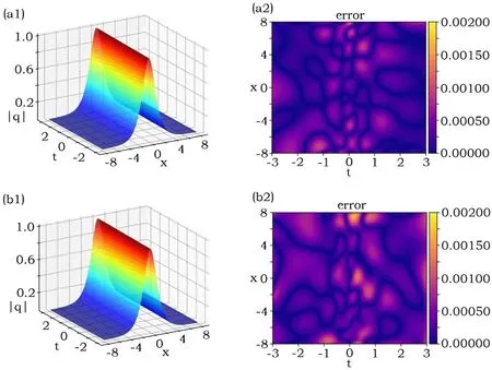
Figure 6.Data-driven parameter discovery of μ and ν in the sense of bright soliton(7).(a)(b)display the learning result under bright soliton data set.(a1)–(a2)are calculated without perturbation.(b1)–(b2)are calculated with 2%perturbation.(a2)and(b2)exhibit absolute value of difference between real solution and the function represented by the neural network.The relative L2- norm error of q(x,t),u(x,t)and v(x,t),respectively, are (a1)–(a2) 8.0153 × 10-4, 1.0792 × 10-3, 1.2177 × 10-3, (b1)–(b2) 1.0770 × 10-3, 1.6541 × 10-3, 1.3370 × 10-3.

Acknowledgments

This work is supported by the National Natural Science Foundation of China (Nos.11 925 108 and 11 731 014).