Tomography of emissivity for Doppler coherence imaging spectroscopy diagnostic in HL-2A

Bingli LI(李兵利),Tianbo WANG(王天博),Lin NIE(聂林),Ting LONG(龙婷),Zijie LIU(刘自结),Hao WU(吴豪),3,Rui KE(柯锐),Zhanhui WANG(王占辉),Yi YU (余羿), and Min XU (许敏)

1 Southwestern Institute of Physics,Chengdu 610041,People’s Republic of China

2 University of Science and Technology of China,Hefei 230026,People’s Republic of China

3 Department of Applied Physics,Ghent University,9000 Ghent,Belgium

Abstract A newly developed Doppler coherence imaging spectroscopy (CIS) technique has been implemented in the HL-2A tokamak for carbon impurity emissivity and flow measurement.In CIS diagnostics,the emissivity and flow profiles inside the plasma are measured by a camera from the line-integrated emissivity and line-averaged flow,respectively.A standard inference method,called tomographic inversion,is necessary.Such an inversion is relatively challenging due to the ill-conditioned nature.In this article,we report the recent application and comparison of two different tomography algorithms,Gaussian process tomography and Tikhonov tomography,on light intensity measured by CIS,including feasibility and benchmark studies.Finally,the tomographic results for real measurement data in HL-2A are presented.

Keywords: Bayesian inference,Gaussian process tomography,HL-2A,Tikhonov tomography,CIS

1.Introduction

In recent years,the Doppler coherence imaging spectroscopy(CIS)diagnostic has been gradually applied on various fusion devices to study impurity issues in the scrape-off-layer(SOL)and divertor[1–3].Its main advantages over the conventional grating-based spectrometer are the high throughput and its ability for 2D measurement via Doppler shifts of ion emission lines using an imaging interferometer [4–6].On the other hand,the information extracted from spectroscopy is lineintegrated for emissivity and line-averaged for particle flow along the line of sight.Therefore,the local emissivity and flow of particles need to be inferred with tomographic inversion methods.However,for flow inversion,this task is challenging; at present,it is beyond the frame of this contribution,which is focused on emissivity reconstruction only.

From a mathematical point of view,the tomography problem is an estimation of the quantity of interest from the measured line-integral signals[7].This is a classical ill-posed problem,for which there is no unique solution because of the finite sampling,and a differential operator in the inversion amplifies noise present in the input data [8].A variety of alternative algorithms have been proposed to solve this problem,some of which are quite well known,such as the Tikhonov regularization method [9,10],minimum Fisher information,etc [11].These methods mainly involveχ2optimization with different regularization constraints.

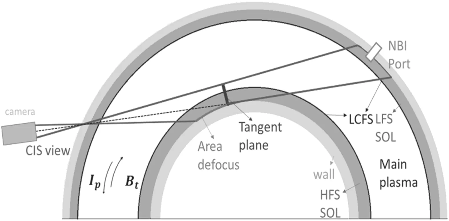
Figure 1.Top view of CIS field of view in HL-2A tokamak.

However,given the large datasets and complicated models,a newly developed approach to the line-integrated modeling challenge is Bayesian inference in fusion plasma[12–14].The Bayesian inference methodology,which comes from the machine learning field,describes the relevant knowledge and targeted unknowns in probability form.It starts with the priori probability,the state of knowledge about the priori information,such as smoothness.Then it is modified by the experimental measurements through the likelihood probability and yields the posteriori probability,which could qualitatively describe the inference result and uncertainty.These will be discussed in detail in section 3.Different from regularization approaches,Bayesian inference is based on probability theory,and the inference is to find the best estimate from all the possible distributions.One of the benefits of this analysis is that the random errors and systematic uncertainties are an intrinsic part of the analysis rather than an afterthought.Furthermore,the prior knowledge,including known parameter interdependencies,is made explicit [15].Bayesian inference has been widely implemented in many complex physics problems,such as astronomy,neutron analysis,etc [16,17].

In this article,the content has been organized as follows:section 2 presents a brief description of the CIS diagnostic in HL-2A.In section 3,we give an overview of the tomography problem,followed by the mathematical formalism of Bayesian inference and Tikhonov regularization tomography.The validation of the method using synthetic data,namely the phantom test,is described in section 4.The results and conclusion are presented in sections 5 and 6,respectively.

2.Doppler CIS in HL-2A

The HL-2A tokamak is a medium-sized magnetic confinement device with a major radius of 1.65 m and a minor radius of 0.4 m [18].The CIS system was put into operation in the latest campaign of HL-2A (2018–2019) and used for the imaging of CIII lines emitted from the plasma SOL on the high-field side (HFS) [4].The observation central axis has been ranged tangentially to the toroidal magnetic field.The top view of this is shown in figure 1,where the complex optical elements are omitted.The light emitted from carbon impurities passes through the lens and waveplate,which imposes an additional phase delay,eventually interfering at the image plane at the phantom V2012 high-speed camera.The distance from the visible surface to the camera is 1884 mm,with the depth of field being ～100 mm.The spatial resolution in the horizontal direction is then estimated to be up to ～0.8 mm.The spatial resolution in the vertical direction is determined by the scale of the fringes,which is ～11 pixels per fringe.So,the spatial resolution in the vertical direction is estimated to be up to ～9 mm,and the field of view is ～34°.Limited by the field of view,the viewing sight is mostly concentrated on the HFS,while the shapely imaged object plane is ～927 × 580 mm2.

The principle of the extracting flow and emissivity from the interferogram has been described in detail in [19,20].Without considering the attenuation and other optical characters,the emissivity and flow extracted from the interferogram are the line average and line integral along the diagnostic line of sight inside the vacuum vessel.

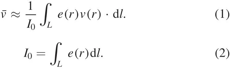
The aim of inversion is to estimate the local emissivitye(r)and local flowv(r)of a particle from the integral intensityI0and averaged flow.Flow inversion is challenging (two variables and one dot product),so at present it is beyond the frame of this contribution,which is focused on emissivity reconstruction only.Before inversion,the plasma region needs to be discretized.Because the line of sight is tangential to the toroidal magnetic field direction,the plasma imaging region to invert is three-dimensional (3D).A simple approach to discretize the 3D region is using the cube grid,i.e.the voxels in figure 2(a).The emissivity in every voxel is assumed to be uniformly distributed.The voxel size is about 10 mm×8 mm×0.1 rad in theR,Zand toroidal direction,respectively.The lines of sight pass through these voxels and are cut into many small pieces.These line pieces form the response matrixRm×n,whose elementsRi×jrepresent the length of sight lineithrough voxelj.Under the assumption of toroidal symmetry,the emissivity field is the same in every toroidal plane.A single 2D inversion could be achieved by integrating the line length along the toroidal direction,which could reduce the size of the response matrix by more than one order of magnitude.Figure 2(b)shows that some lines of sight cross the toroidal (R,Z) plane,which is curved due to the shape of the vacuum vessel,while the integral equation (2)with measurement uncertainty could be inverted into

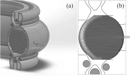
Figure 2.(a)3D diagram of sight lines and voxels in vacuum vessel.(b) Display sight and grids in the R-Z plane.The sight line is integrated to 2D and the line of sight is curved due to the assumption of toroidal symmetry.

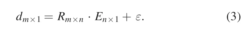
En×1is the vector of local emissivity in voxels andεdenotes the error term to account for measurement uncertainty; it is often assumed as probabilistic independent and identically follows Gaussian probability distribution.The inverse problem is to estimateEn×1according to the detection datadm×1.

3.Plasma tomography

To solve this inversion problem,a variety of well-established mathematical methods have been developed,most of which could be achieved by regularization,e.g.Tikhonov regularization,minimum Fisher information regularization,etc.However,from the perspective of probability theory,Bayesian inference provides a probability distribution of the physical parameters rather than a single solution.In theory,we could obtain the most likely solution and quantify the uncertainty of this solution.

3.1.Bayesian inference

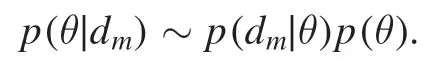
Estimating the unknown quantity from the measurement,Bayesian inference is a powerful method from the perspective of probability.Before the measurement,there already exists certain prior knowledge about the distribution emissivity field.The state of knowledge could be described as the prior probabilityp(En).This is updated through the Bayesian theorem as data become available.

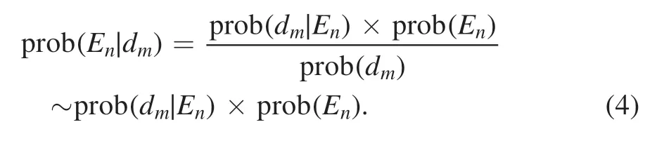
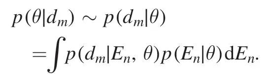
The likelihood term prob(d m∣En)measures the mismatch between the measured line integrals and their predictions given the assumption of some emissivity field.The evidencep(dm)could be considered as a normalization factor because it does not explicitly depend on the emissivity,so it could be omitted,and the equality is replaced with proportionality.These constitute the posterior probability functionp(E n∣dm).The posterior probability function quantifies our uncertainty on the estimated emissivity field,given the model,prior knowledge and the measured data,and it represents the probability for all possible results.

3.2.Gaussian process tomography

In Bayesian inference,the selection of prior information is important.There is an infinite set of possible functions,and the prior information is always accompanied with the inference result,which would be updated by measurement data in the end.If the available data are not sufficient,the choice of prior becomes even more important.This is where the Gaussian process comes to the rescue.Gaussian process tomography(GPT)is a newly developed method[21–23]that makes use of the Bayesian framework,especially in the selection of the prior.In GPT,the prior is set as a Gaussian process probability density function,which is a kind of generalized multivariate normal distribution space.It is described by a mean functionμand a covariance function Σ.In our application of CIS tomography,whereGP～N(μ,Σ),it means that the probability density function of local emissivity in every cell follows a Gaussian distribution,while the joint distribution of every subset of voxels is multivariate normal.The covariance function describes the relation among these voxels.In other words,the emissivity in different voxels has a certain correlation and should stay in a proper smooth distribution.The smaller the distance between voxels,the greater the correlation.According to the simulation results of the UEDGE simulation [6],carbon impurities move along the magnetic field line.So,the correlations parallel and perpendicular to the magnetic field line are different.This relationship can be expressed by the squared-exponential kernel function

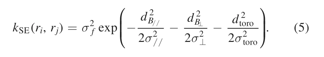
Here,ri,rjare the voxel center coordinate positions in voxelsi,j,respectively.dB//anddB⊥represent the vertical and parallel distance along the magnetic field line between two voxels,respectively,whendtorois the toroidal physical arc length.The kernel function depends on four parametersσf,σ//,σ⊥andσtoro,called hyperparameters in Bayesian terminology,and they determine the correlation between emissivity in different voxels or the smoothness of the emissivity field in different directions.A discussion on how to choose suitable hyperparameters can be found in appendix A.Under the assumption of toroidal symmetry,the smoothness along the toroidal direction is infinite.In other words,σtorois infinite and the termin equation 5 can be omitted,and the 3D inversion problem can be transformed into a 2D problem.The relationship between different voxels forms a covariance function of Gaussian distribution:

Figure 3.Phantom emissivity fields set by Gaussian density function in our tests.(a)A single peak,(b)two symmetrical peaks,(c)two peaks in the top half,(d) complex structure.

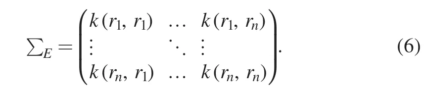
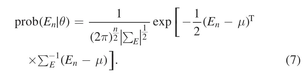
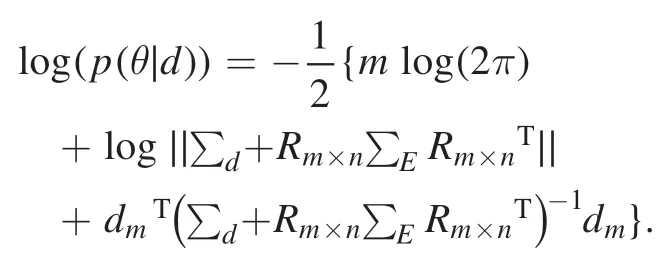
Here,k(ri,rj)=cov [E(ri),E(rj)],withE(ri),the emissivity in pixeli,is the covariance kernel function whileE(ri) is the emissivity in pixeli.Then we can obtain the prior probability Here,is the prior mean,which will be fixed at 0,or it may be chosen on the basis of earlier experiments or expert knowledge.Experimental measurements modify current probability or knowledge through the likelihood function(d m∣En,θ).It means that given the emissivity feild,we can obtain the probability of the measurement data.Assuming the measurement error in forward function (dm=Rm×n·En+ε) follows Gaussian distribution,the likelihood can be written as

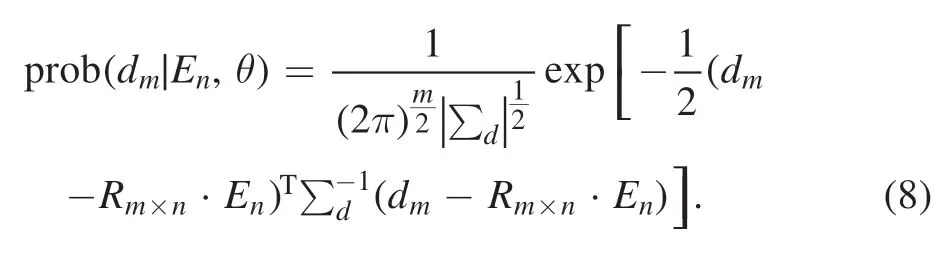
Here,∑dis the covariance function of the measurement data,describing the measurement uncertainty and correlation on the vectordmof measurement line integrals.We assume that the various line-integrated measurements are independent and choose a 5% noise level.

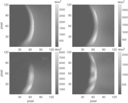
Figure 4.Simulated detection data obtained from phantom tests.(a)A single peak,(b)two symmetrical peaks,(c)two peaks in the top half,(d) complex structure.

Finally,the posterior probability could be obtained.One of the major advantages of choosing the Gaussian process as the prior probability is that the posterior is also a Gaussian function.The mean vector and covariance matrix can be obtained directly,and the inference result can be obtained extremely quickly.

3.3.Tikhonov tomography

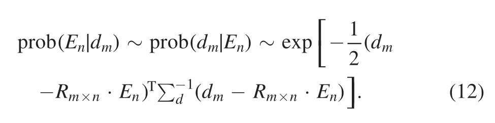
Tikhonov tomography is one of the most successful methods applied in fusion tomography studies,especially in JET,and has been in use for over 20 years.On the other hand,this inference method can also be derived from Bayesian inference.If the prior is treated as a constant,the posterior is proportional to the likelihood,and the constant term can be omitted:

The maximum of the posterior is the same as the leastsquares equationwhich stands for the data fidelity.As assumed above,∑dis the covariance matrix,and if we make a further assumption,it can be weighted todmandEnby a square root of the covariance matrix [24]

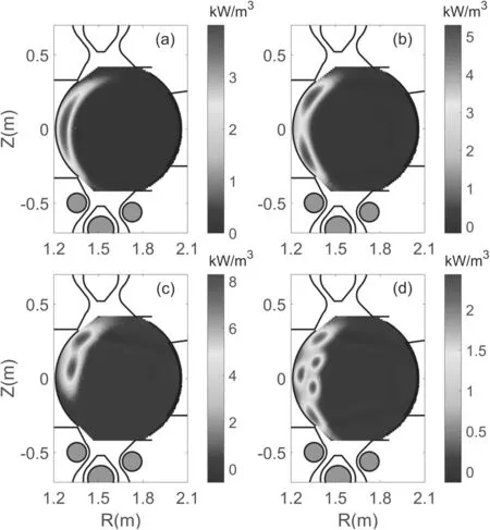
Figure 5.The tomographic results with Bayesian method on phantom data.(a)A single peak,(b)two symmetrical peaks,(c)two peaks in the top half,(d) complex structure.

However,the solution is too sensitive to the measurement value,which leads to large errors with the ill-posed problem.A common solution to find a unique and sensible solution in the general form is to add Tikhonov–Philips regularization[25]:

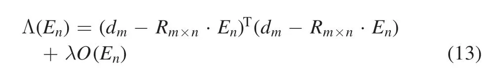
where ( )O Enis the regularization function andλis a hyperparameter,which can balance the strength of prior constraints with the goodness of fitting.The most common regularization operators are the identity operator and Laplace operator[23,26].According to the character of the emissivity field,we choose the Laplace operator:

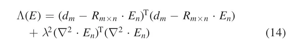
∇2is the Laplacian operator,which can be written as a matrixC.The elements of the matrix are shown in the following equation:

HerenRis the voxel number along theRdirection.In fact,the purpose of ( )O Enis to imposea prioriknowledge on the emissivity,which is often some kind of a roughness penalty and a boundary constraint.The minimum reached by derivation

According to this,a direct inversion of this equation is possible.However,before this,the choice of the optimal parameter λ is one of the key issues related to Tikhonov regularization.Since the wealth information extracted from CIS diagnostics are sufficiently rich,theL-curve are available to choose a suitable λ[27],which is described in appendix B.

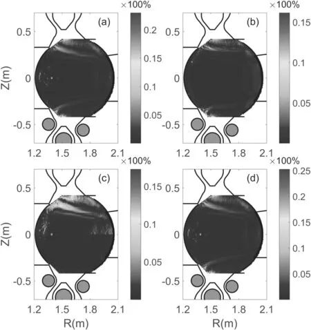
Figure 6.Error map with Bayesian tomography method on phantom data.(a)A single peak,(b)two symmetrical peaks,(c)two peaks in the top half,(d) complex structure.

There are many other regularization methods,such as minimum Fisher information[28],maximum entropy method,etc [29].Some of these are solved iteratively.In some cases,prior information such as positivity and bound constraints is allowed to be imposed at each of the iterations,which is applied in the CIS system on DIIID and MAST [5,6].However,the role of prior information is not as explicit as the probability method.

4.Phantom tests

In order to review the performance of the tomographic algorithm,we have performed a phantom test,which uses the Gaussian probability density function to generate synthetic models similar to the distribution of impurity particles.Then we send the synthetic measurement to tomography code to get the reconstruction results and compare the differences between the reconstruction and presets.For CIS in HL-2A,the diagnostic viewing field is mainly oriented on the HFS,thus the synthetic distributions are mainly set on the HFS.As shown in figure 3,four different shapes were used for the phantom test:one peak,two symmetrical peaks,two peaks in the top half,and a complex shape.

Then,forward models of line integrals were calculated on 120×120 pixels,which amounts to the simulation camera data as shown in figure 4.There are some glitches and spatial aliasing near the peak that may be caused by data discretization.Increasing the number of voxels could decrease the scale and number of glitches.While satisfying the computation power,it is best to make the number of voxels as large as possible.

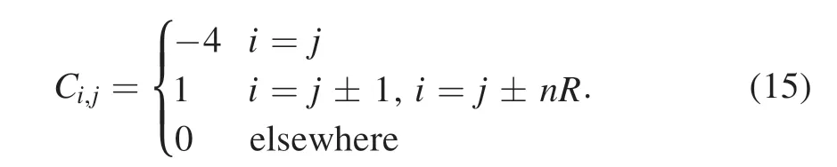
Then the simulation camera data with 5%noise level was made tomography and the reconstructed results could be in comparison with the models data set.Besides noise,systematic errors may considerably damage the ill-posed task and were tested in section 5.The quality of the reconstructions can be quantified through a relative error map,showing the difference between the phantom and reconstructed field,normalized by the maximum phantom emissivity

Figure 7.The tomographic results with the Tikhonov method on phantom data.(a)A single peak,(b)two symmetrical peaks,(c)two peaks in the top half,(d) complex structure.

4.1.GPT method test

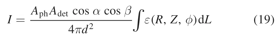
Firstly,the GPT method was tested with a 5% noise level.The results and errors are demonstrated in figures 5 and 6,respectively.The reconstructed emissivity field can be easily distinguished and the maximum relative error is about 24%,17%,16%and 25%.Among these,the area near the wall in the bottom left and top left corners,where the line of sight is hard to reach,accounts for most of the error.Aside from these areas,the maximum relative error decreases to about 10%except in figure 6(c).

4.2.Tikhonov tomography method test

Similar to GPT tomography,the Tikhonov method’s performance was evaluated with a 5%noise level phantom test.The results and errors are shown in figures 7 and 8,respectively.The results are similar to those of GPT tomography.The maximum relative errors are a little larger than 24%,24%,19% and 26%,respectively.The error is still concentrated in the area near the wall,but the error of the other region is larger than that of the GPT method.

4.3.3D attempt

In the previous section,we transformed the 3D problem into a 2D one.The principle is very simple.The emissivities in a row of voxels along the toroidal direction are assumed to be the same,ET1=ET2=ET3……ETn=ET,under the assumption of toroidal symmetry.The contributions of these voxels to pixeliof the camera are(ET1Ri,T1+ET2Ri,T2……+ETn Ri,Tn)=ET(Ri,T1+Ri,T2……+Ri,Tn) =ETRi,T,so the 2D element of the response matrix is just the integral of the length of the line of sight along the toroidal direction.The line of sight becomes a curve in 2D due to the assumption of toroidal symmetry,as shown in figure 2.In other words,if the influences of optics and other factors are not considered,these voxels could be regarded as one voxel along the toroidal direction.

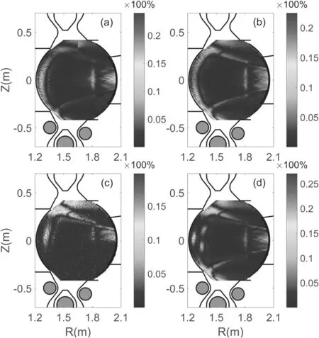
Figure 8.Tomographic error with the Tikhonov method on phantom data.(a)A single peak,(b)two symmetrical peaks,(c)two peaks in the top half,(d) complex structure.

At present,it is hard to deliver a reliable 3D reconstruction with the present available diagnostic conditions.First,the great numerical calculation is extremely costly.Second,the regional coverage of one single camera is limited,and some information is lost(for example,the impurity ion on the LFS (the low-field side)).On the other hand,if there were more cameras available,it would be more feasible and reliable to make 3D tomographic reconstructions.If the above two issues could be resolved,a reliable 3D tomography reconstruction would be achievable.Furthermore,in the Bayesian inference methodology,the tomographic result of one diagnostic could be used as prior information for other analyses;multiple diagnostics could be considered comprehensively and deliver an integrated inference.As a consequence,we make a 3D attempt at this problem under the assumption of toroidal symmetry.The GPT result is shown in figure 9.The result seems acceptable,so we believe Bayesian inference may be useful in future 3D inversions.

According to the above results,the reconstruction error is mainly focused on the area near the wall,where the number of lines of sight is fewer compared to that in the other area.The measurement did not provide enough information to infer a more accurate reconstruction.On the other hand,the carbon impurities are mainly distributed within the SOL,which is close to the edge.This should be improved in the future diagnostic upgrade with more lines of sight.It can be noted that if the camera viewing direction was modified to a better angle(up or down),the quality of the corresponding position inversion may be greatly improved.Moreover,the relative error is less than 10% in the present reconstruction,which is still acceptable.

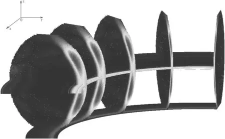
Figure 9.Tomographic 3D results with GPT method on two symmetrical peak shape phantom data.

Figure 10.Schematic diagram of Gaussian imaging.When the light point source is far from the objection plane,the light collected is no longer a point but a 2D distribution.

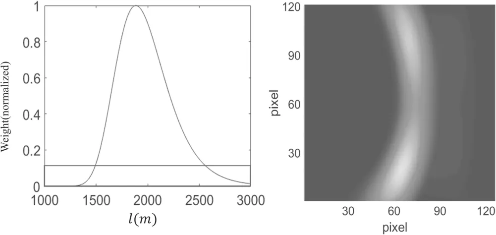
Figure 11.Exponential decay with the distance from the focus and forward model result.

5.Error source study

Although both tomography methods produce good results with artificial data,there are always unexpected mistakes when dealing with practical problems,because there are many problems that need to be simplified or even ignored.Furthermore,we could not gain the true distribution of impurities in order to gain the error and analyses.So,we should consider various factors that cause errors and decide whether to ignore or simplify these factors,such as certain optical characteristics,data discretization,viewport misalignment and the level of noise.

5.1.Optical factors

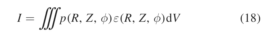
Due to the camera diagnostic,the information extracted from the image is affected by certain optical characteristics.The first factor to consider is line-integral approximation.Strictly speaking,the signal measurements from CIS result from volume integrals.The powerImeasured by a detector aperture from infinitesimal volumeVd can be expressed as whereε(R,Z,φ)is the emissivity in the voxels andp(R,Z,φ)represents the detector point response function,merely the solid angle of a point in the specified volume element subtended by the area of the detector element,optical contribution of point light source in voxels to detector.For a detector of infinitesimally small area collimated by a simple pinhole with effective areaAph,the solid angle viewed iswheredis the distance between the detector and pinhole.A real detector has a finite area but as long as the field of view is narrow (dΩ≪1,in HL −2A dΩ≈0.01),the power incident on a detector from a volume element of plasma could be considered to be looking along the same chord [30]:

whereAdetis the area of the detector,αis the angle between the normal direction of the detector and the chord,andβis the angle between the normal direction of the pinhole and the chord.

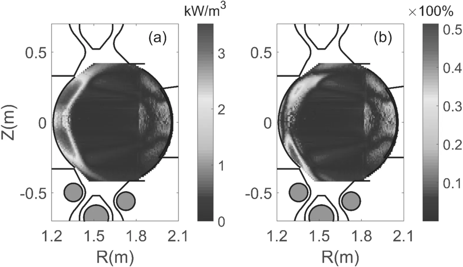
Figure 12.The results (a) and error map (b) of two symmetric peaks when position shift occurs by 20 mm in the horizontal direction and 5 mm in the vertical direction.

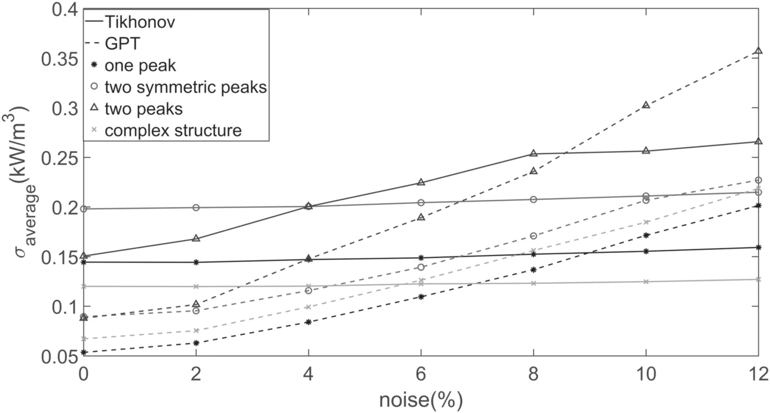
Figure 13.The change ofσaverage with the level of noise.The dashed lines are the results with GPT while the solid lines are the results with the Tikhonov method.Different symbols stand for different models.

The point spread function (PSF) is another optical factor to be considered.As figure 10 shows,the light emitted from an infinitely small ideal point source on the objection plane would be collected as a point by the delector.However,if the source deviates from the objection plane,the light collected by the delector is a 2D distribution rather than an ideal point signal as figure 10 shows; many researchers thought it was Gaussian distribution; Gaussian distribution is accepted by many researchers[31].When the light source continues to be far away from the object plane,the light is more dispersed until it exceeds the resolution of the pixel,namely the depth of field.By the way,even the ideal point source in the objection plane,what the detector detects is still a scattered light due to the wavelength of light.In addition,the flow of the plasma,the aperture,etc would cause the PSF.As figure 1 shows,the plasma on the HFS to reconstruct is beyond the depth of field,so it needs some processing.

For inversion,the diffusion on the detection of the light is difficult to calculate.However,according to the model above,far away from the center,the light intensity decreases exponentially.So it was assumed not to diverge on the detector but to decay exponentiallywhich is similar to the general deconvolution method to deal with PSF.I0is the intensity of light without considering the PSF,lAis the distance from the object surface to the camera andlBis the vertical distance from the point in the voxels to the camera,which is shown in figure 11(a).σis determined by the camera parameters.To avoid the impact of data instability,we omit some cells with the weight lower than the threshold marked by the red line in figure 11(a).

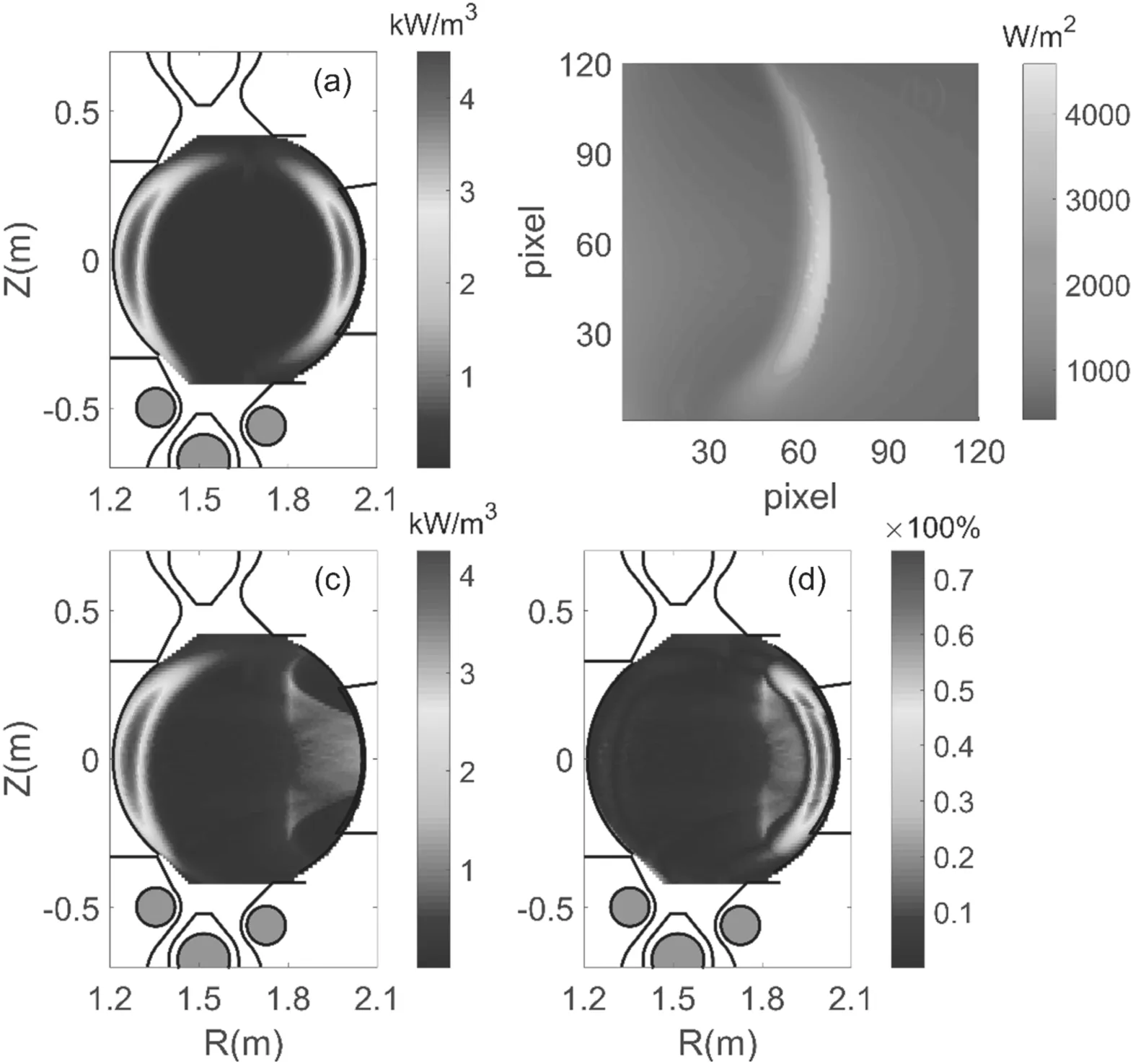
Figure 14.Influence of the emissivity with CIII impurities on LFS.(a) Model of CIII impurity ions distributed on HFS and LFS,(b)simulation detection data,(c)tomographic results with the Tikhonov method on this model,(d)error map with Tikhonov tomographic result.

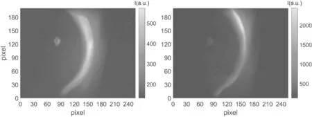
Figure 15.The emissivity field extracted from camera pictures of 1131 ms and 1132 ms for shot 35452.

5.2.Viewport misalignment

In order to be free from mechanical vibration and electromagnetic interference,the detector was fixed on a bracket at least 3 meters away from the device.The measured position of the detector may deviate from the actual position,which causes offset of the calculated magnetic field and possible error in the result.The systematic error on the diagnostic position must be taken into consideration.

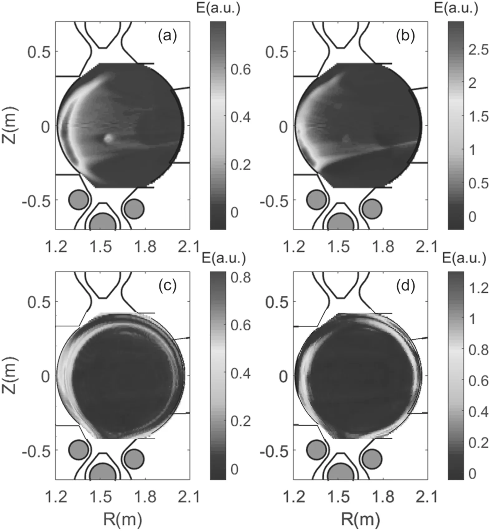
Figure 16.Tomography results.(a)1131 ms,(b)1132 ms for shot 34542 with the Tikhonov method and(c)1131 ms,(d)1132 ms with GPT method.

So,after obtaining the simulation image with the two symmetrical peak shape,we shifted the camera’s coordinates by 5 mm in the vertical direction and 20 mm in the horizontal direction to test the impact of offset on the GPT results.

The results and error map are shown in figure 12.The shape is a bit fuzzy and the maximum relative error increases to about 50% in the main area of impurity distribution and exceeds that in the area near the wall.Fortunately,the Tikhonov method has higher robustness,and the reconstructed results with which seems reasonable.

5.3.Sensitivity to level of noise

The sensitivity of the two algorithms to the level of noise is an issue that has to be considered.In order to quantify and make comparisons with the sensitivity,we define the average error as

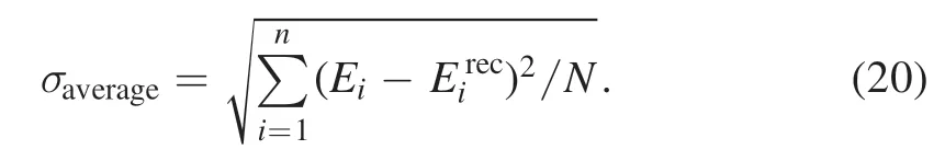
After obtaining the simulation camera data,different levels of independent random noise (2%–12%) were added.The other parameters remain unchanged to obtain the function of average error with respect to the level of noise,as shown in figure 13.The average error of GPT is smaller than that of the Tikhonov method obtained when the noise is at a lower level,but as the noise level increases,the average error of GPT increases more rapidly.When the noise reaches a certain level(above 5% from the figure),the average error of the GPT method exceeds that of the Tikhonov method.In short,if the level of noise is below 5%,GPT could obtain the better results.If the level of noise exceeds this value,it becomes an important factor in model selection.However,the light intensity error in general does not reach this level (～5%,an empirical value).

5.4.Influence of CIII on the LFS

In fact,in addition to CIII in the HFS,CIII are also distributed in the LFS,and the influence of CIII in the LFS on the inversion needs to be tested.The model is set as in figure 14(a); the CIII ions on the HFS and LFS are asymmetric because their settings depend on the magnetic field.Figure 14(b) is the simulation detection through the forward model.Since the CIS diagnostic field of view is focused on the HFS,CIII ions on the LFS cannot be imaged.

The tomographic results and error map obtained by the Tikhonov method are shown in figures 14(c) and (d).The information on the LFS is insufficient to provide effective inversion,so there are some disorganized shadows on the LFS and the maximum relative error increases to above 70%.The results show that it has limited effect on the HFS.The reconstructed results with GPT are similar to that with the Tikhonov method,so they are not reported here.

6.Tomography with CIS experimental data

The intensity extracted from the camera picture of 1131 ms and 1132 ms for shot 35452 is shown in figure 15.It should be noted that the quantity in the paper is just a relative quantity,so it uses arbitrary units.The size of pixels of the camera is 1280 × 800,in order to reduce the size of the required response matrix,the pixels were typical binned at 5 × 4 to 256×200,which is enough to make tomography according to phantom data.The scale of voxels in the (R,Z) plane is about 8 mm ×10 mm.Figures 16(a) and (b) show the results of using the Tikhonov method.There are a lot of carbon ions in the central area of the plasma,which may be caused by the optical properties not being completely handled.

In theory the GPT method,as shown in figures 16(c)and(d),should gain better results with more hyperparameters;however,the result is not as good as that obtained with the Tikhonov method,which may be caused by the offset of the coordinates.As a result,the optimization of hyperparameters becomes more difficult and the results become very volatile and may be far from the true distribution,as figures 16(c)and(d)show.The coordinates of the camera need to be rigorously calibrated in subsequent experiments.

7.Conclusion

In this paper,two CIS tomography algorithms,the GPT and Tikhonov methods,for emissivity in HL-2A have been introduced.In comparison with traditional tomography techniques,e.g.the Tikhonov tomography method,the GPT method has several advantages.First of all,the connection between prior information and measurement data is made explicit.Secondly,the random errors and systematic uncertainties are an intrinsic part of the analysis rather than an afterthought.The results of one diagnostic could be the prior information of another,so multiple diagnostic data can be considered comprehensively.

Besides the error caused by the algorithm,many factors that influence the error have to be considered,such as optical characteristics,viewport offset,etc.For real datasets,the Tikhonov method is more robust and gives a more reliable result than GPT in our experiment because of the systematic errors caused by equilibrium information.With the completion of HL-2M construction,the CIS position will be calibrated strictly,then we believe the reconstructed results of GPT would be greatly improved.

Acknowledgments

This work was supported by the National Key R&D Program of China (No.2019YFE03040004) and National Natural Science Foundation of China (Nos.12005052,11905050,U1867222 and 11875124).

Appendix A.GPT hyperparameter optimization

The choice of suitable hyperparameters is a key issue using both the GPT and Tikhonov methods.As mentioned above,these hyperparameters determine the degree of smoothness of the reconstructed emissivity field.The optimal parameters should minimize the difference between the reconstructed and the original profiles.Since the original profiles were not available in the experiment,these parameters have to be determined from the measurements and prior knowledge by Bayesian inference.Similar to the posterior forEn,the posterior for hyperparametersθcan be written as

Now,if we assume a non-information uniform hyperprior distribution ( )θp,the posterior for hyperparameters is proportional to the evidence of the emissivity field as follows

With equation (8),this results in the following expression to make the maximum of the above formula

In fact,choosing suitable hyperparameters for the GPT method is hard due to four parameters,or three in 2D.Intelligent algorithms also often fail due to matrix computation.However,these parameters can be set in a certain range,such as non-negative according to prior knowledge to reduce the difficulty of searching.

Appendix B.Regularization parameter

In Tikhonov regularization,there are many different methods proposed to solve this problem,such as Morozov’s discrepancy[32],the curvature of theL-curve[7,33],and so on.Here,the common method,the curvature of theL-curve,was chosen to optimizeλ.First of all,we start with the singular value decomposition

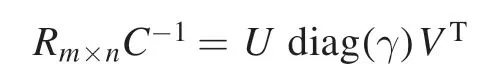
whereU∈RM×NandV∈RN×Nare orthonormal matrices and(γ)diag is a diagonal matrix withmelements.If we define a vector

the residual normρ2and seminormη2based on singular value decomposition are defined as

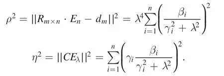
The error of the solution in Tikhonov regularization is composed of two parts:the ill-posed matrixLand the regularization term.So,the optimization minimizes both the regularizationη2and the residual term of the equationsρ.2 Plottingρ2andη2in the logarithmic axis,the shape of the curve is likely to be L-shaped.In general,λoptis located at the corner,which balances the ill-posed equation and regularization.