AN UPBOUND OF HAUSDORFF’S DIMENSION OF THE DIVERGENCE SET OF THE FRACTIONAL SCHRDINGER OPERATOR ON Hs(Rn)∗

(李丹)

School of Mathematics and Statistics,Beijing Technology and Business University,Beijing 100048,China E-mail:danli@btbu.edu.cn

Junfeng LI (李俊峰)†

School of Mathematical Sciences,Dalian University of Technology,Dalian 116024,China E-mail:junfengli@dlut.edu.cn

Jie XIAO (肖杰)

Department of Mathematics and Statistics,Memorial University,St.John’s NL A1C 5S7,Canada E-mail:jxiao@math.mun.ca

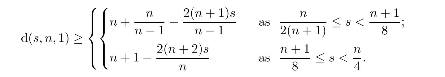
Abstract Given n≥2 and,we obtained an improved upbound of Hausdorff’s dimension of the fractional Schrödinger operator;that is,.

Key words The Carleson problem;divergence set;the fractional Schrdinger operator;Hausdorff dimension;Sobolev space

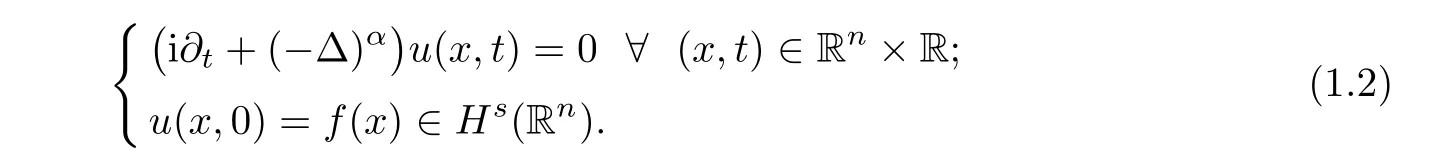
1 Introduction

1.1 Statement of Theorem 1.1

Suppose that S(R)is the Schwartz space of all functions

f

:R→C such that

If(−∆)

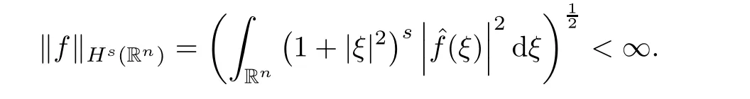
f

stands for the(0

,

∞)∋

α

-pseudo-differential operator de fined by the Fourier transformation acting on

f

∈S(R),that is,if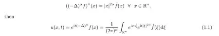

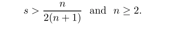
Taking into account the Carleson problem of deciding such a critical regularity number

s

such that

Theorem 1.1

1.2 Relevance of Theorem 1.1

Here,it is appropriate to say more about evaluating d(

s,n,α

).

In general,we have the following development:

Theorem 1.1 actually recovers Cho-Ko’s[1]a.e.-convergence result

as follows:

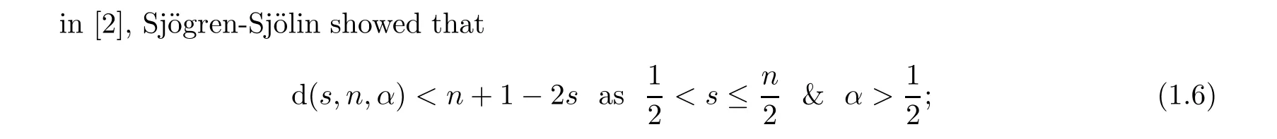
in[3]and[4],it was proved that

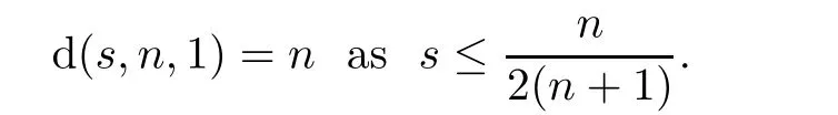
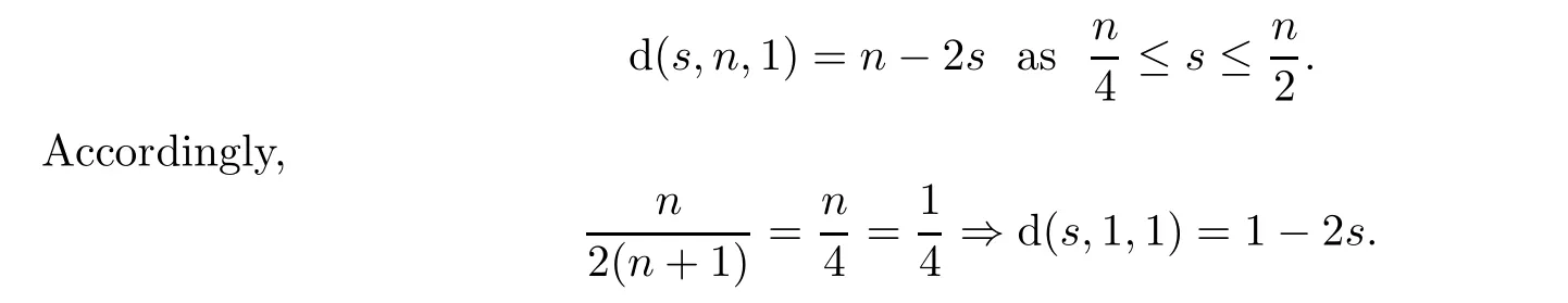
In particular,we have the following case-by-case treatment:

Bourgain’s counterexample in[9]and Luc`a-Rogers’result in[20]showed that

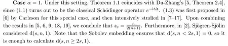
On the one hand,in[5],Du-Zhang proved that

Thus there is still a gap in terms of determining the exact value of d(

s,n,

1);see also[5,20–23]for more information.

Very recently,Cho-Ko[1]proved that(1.3)holds for

2 Theorem 2.2⇒Theorem 1.1

2.1 Proposition 2.1 and its Proof

In order to determine the Hausdorff dimension of the divergence set of

e

f

(

x

),we need a law for

H

(R)to be embedded into

L

(

µ

)with a lower dimensional Borel measure

µ

on R.

Proposition 2.1

For a nonnegative Borel measure

µ

on Rand 0≤

κ

≤

n

,let

and let

M

(B)be the class of all probability measures

µ

with

C

(

µ

)

<

∞that are supported in the unit ball B=

B

(0

,

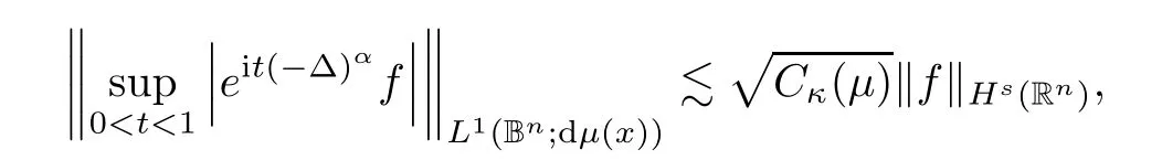
1).Suppose that

(i)If

t

∈R,then

then d(

s,n,α

)≤

κ

.

Proof

(i)(2.1)is the elementary stopping-time-maximal inequality[3,(4)].

(ii)The argument is split into two steps.

Step 1

We show the following inequality: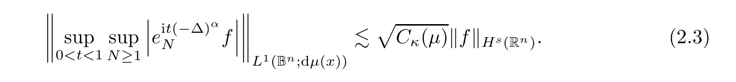

In a similar way as to the veri fication of[3,Proposition 3.2],we achieve

It is not hard to obtain(2.3)if we have the inequalities

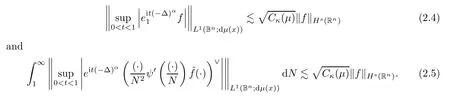
(2.4)follows from the fact that(2.2)implies

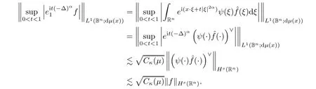
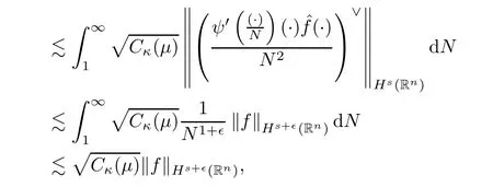
To prove(2.5),we utilize

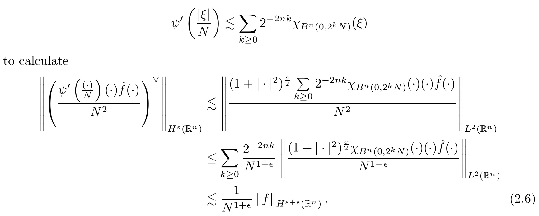
By(2.2)and(2.6),we obtain

thereby reaching(2.5).

Step 2

We now show that

By the de finition,we have

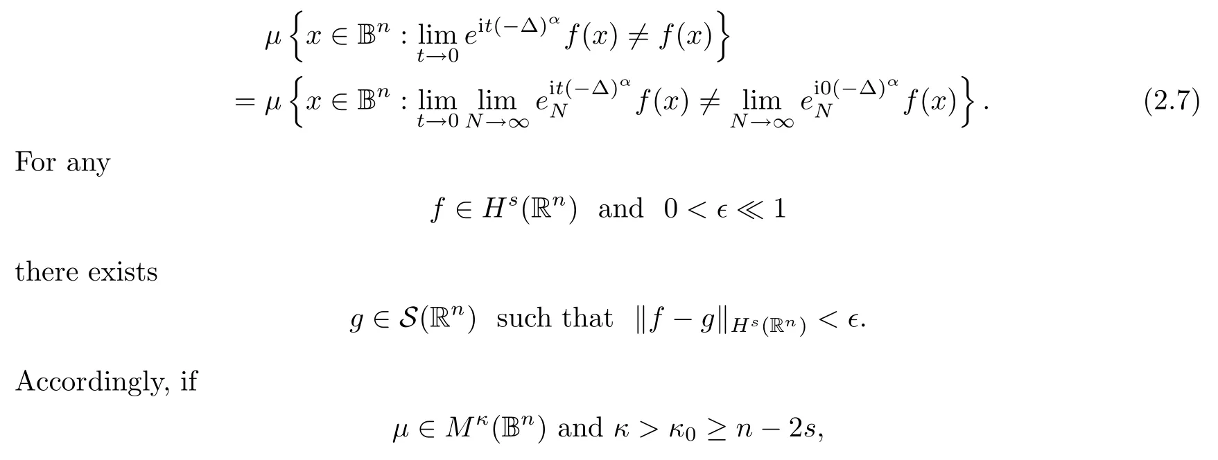
then a combination of(2.3)and(2.1)gives that

Upon first letting

∊

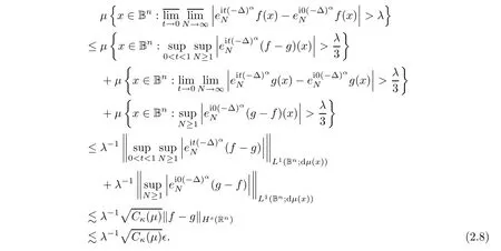
→0,and then letting

λ

→∞,we have

whenever

µ

∈

M

(B)with

κ>κ

.If Hdenotes the

κ

-dimensional Hausdorff measure which is of translation invariance and countable additivity,then Frostman’s lemma is used to derive that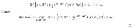

2.2 Proof of Theorem 1.1

We begin with a statement of the following key result,whose proof will be presented in Section 3,due to its nontriviality:

Theorem 2.2

If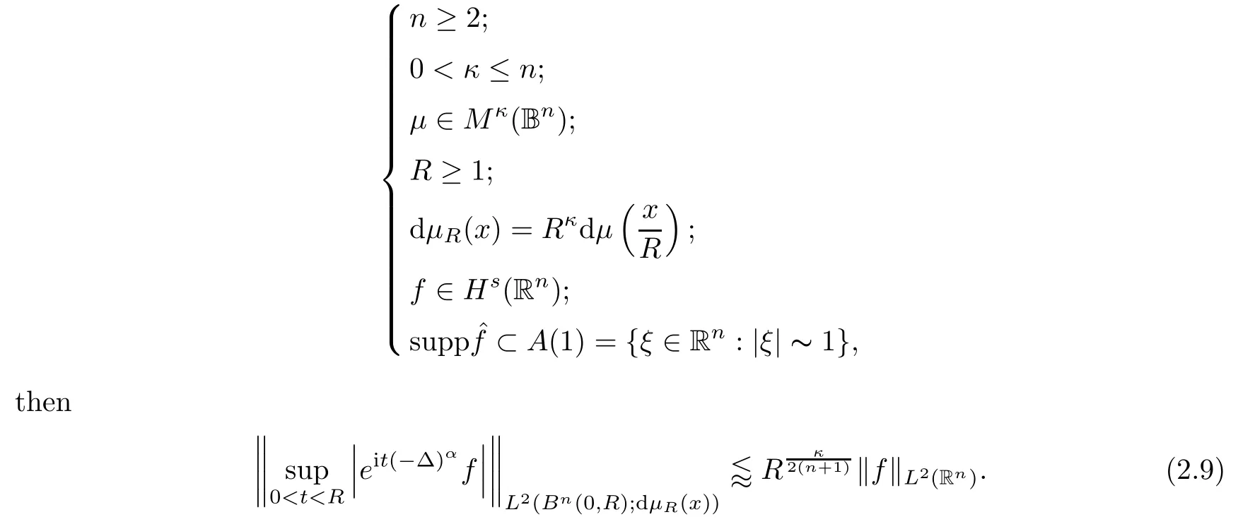

Consequently,we have the following assertion:

Corollary 2.3

If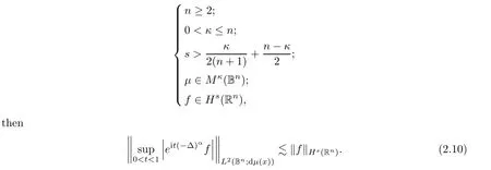

Proof

Employing Theorem 2.2 and its notations,as well as[1](see[10,11,24,25]),we get that

Next,we use parabolic rescaling.More precisely,if

Consequently,if

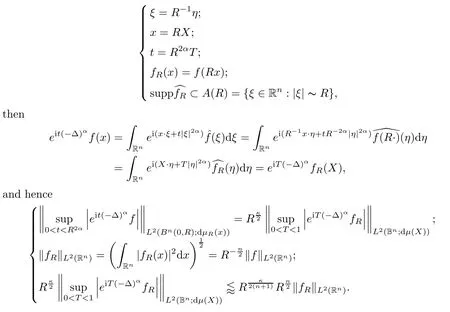
T

=

t

and

X

=

x

,then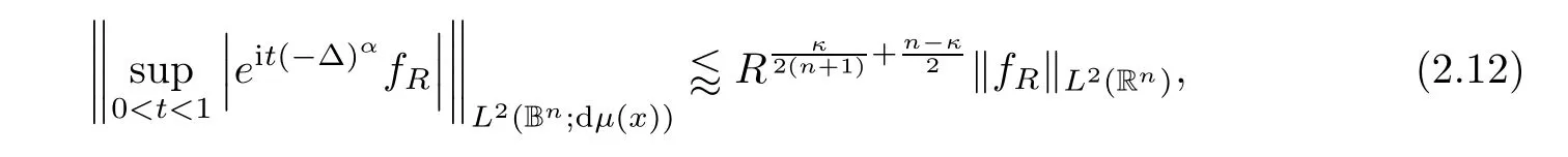

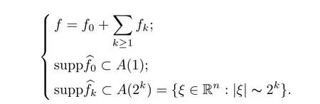
and hence Littlewood-Paley’s decomposition yields that

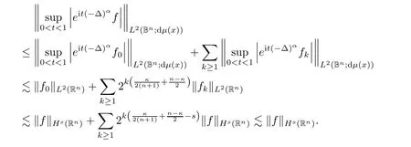
Finally,by Minko wski’s inequality and(2.12),as well as

we arrive at

Next we use Corollary 2.3 to prove Theorem 1.1.

whence(2.2)follows.Thus,Proposition 2.1 yields that

Next,we make the following two-fold analysis:

On the one hand,we ask for

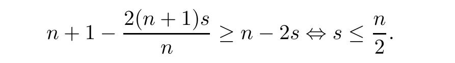
On the other hand,it is natural to request that

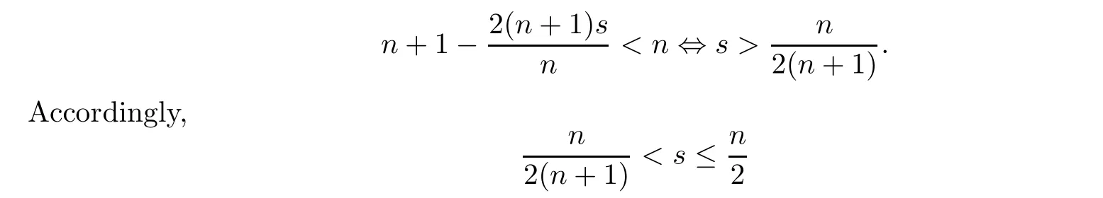
is required in the hypothesis of Theorem 1.1.

3 Theorem 3.1⇒Theorem 2.2

3.1 Theorem 3.1⇒Corollary 3.2

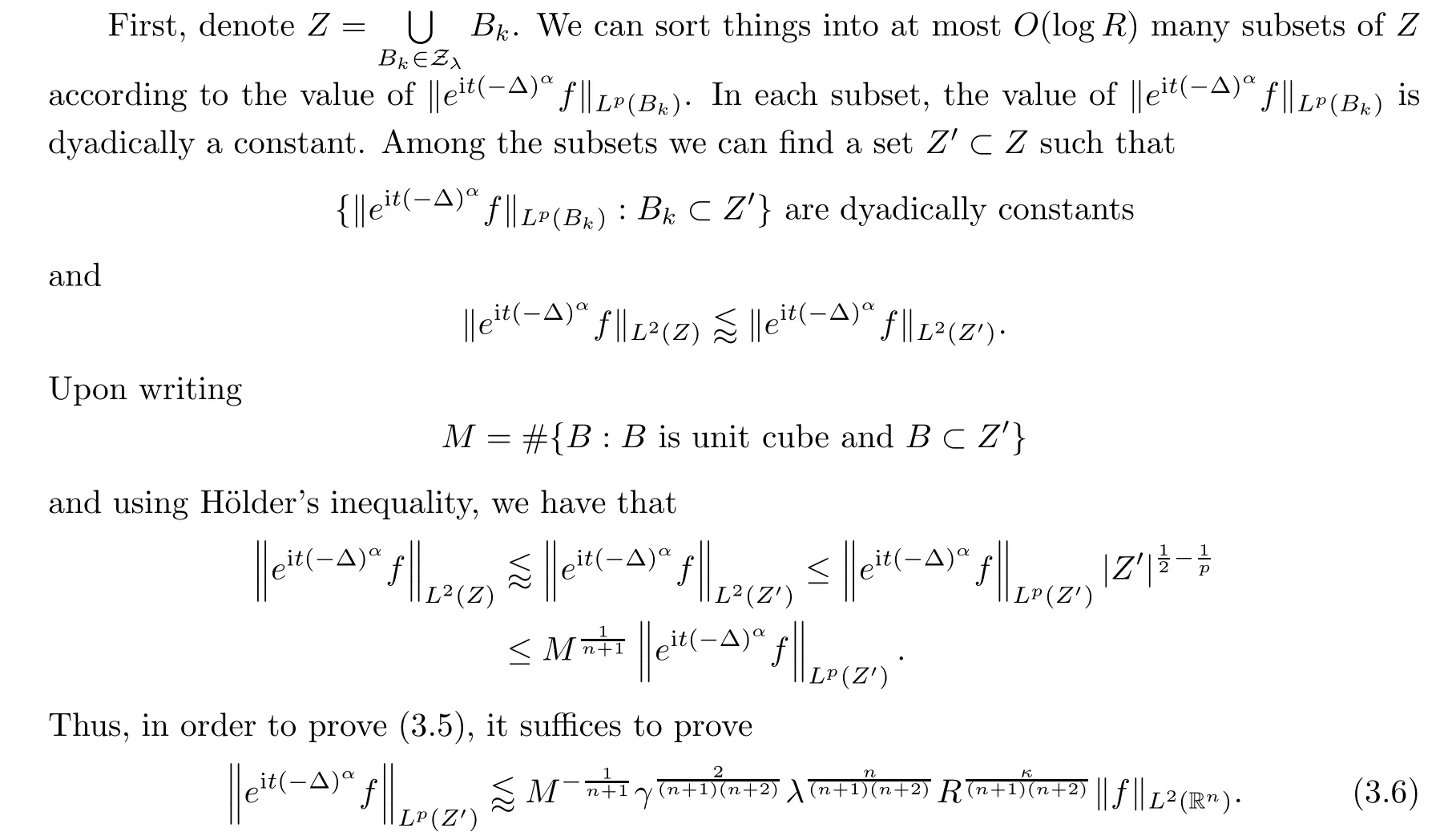
We say that a collection of quantities are dyadically constant if all the quantities are in the same interval of the form(2

,

2],where

j

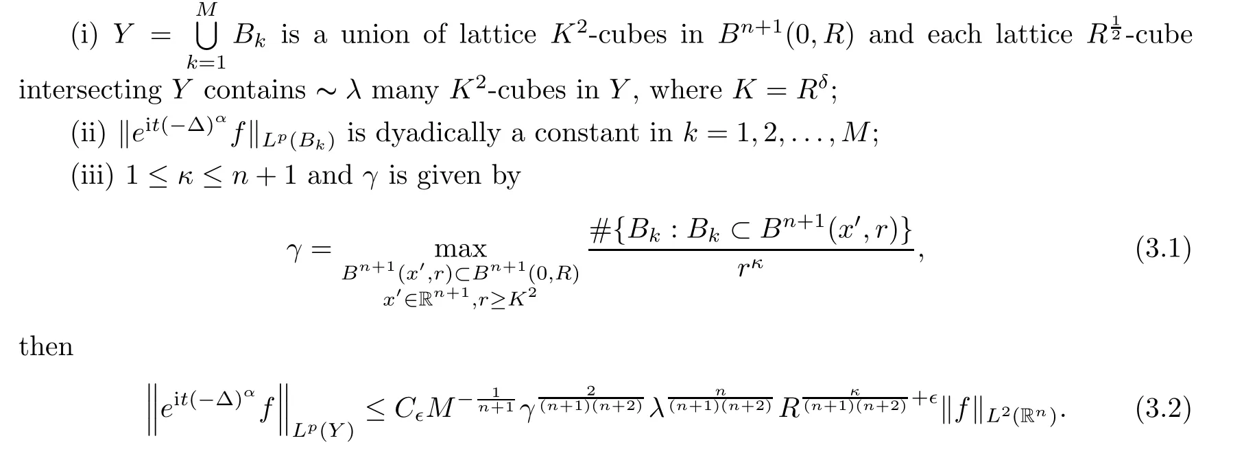
is an integer.The key ingredient of the proof of Theorem 2.2 is the following,which will be proved in Section 4:

Theorem 3.1

Let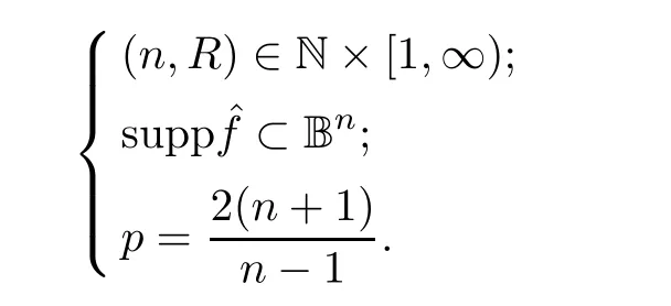

such that if

From Theorem 3.1,we can get the following

L

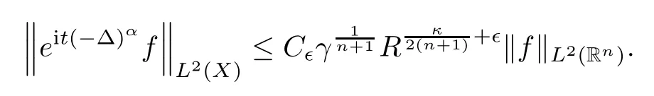
-restriction estimate:

Corollary 3.2

Let

Then,forany

∊>

0,there exists a constant

C

>

0 such that if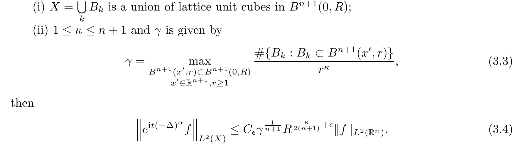

Proof

For any 1≤

λ

≤

R

,we introduce the notation

By pigeonholing,we fix

λ

such that

It is easy to see that

Next,we assume that the following inequality holds(we will prove this inequality later):

We thereby reach

Hence,it remains to prove(3.5).

In order to use the result of Theorem 3.1,we need to extend the size of the unit cube to the

K

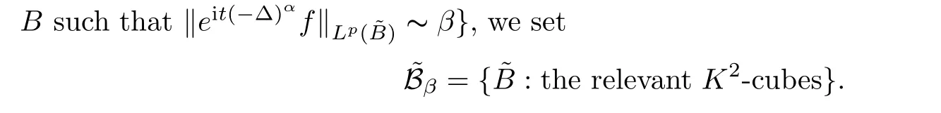
-cube according to the following two steps:

Step 1

Let

β

be a dyadic number,let B:={

B

:

B

⊂

Z

,

and for any lattice

K

−cube

B

˜⊃

Step 2

Next,fixing

β

,letting

λ

be a dyadic number,and denoting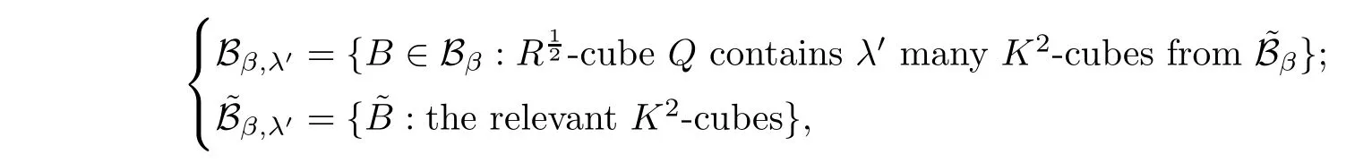

we find that the pair{

β,λ

}satis fies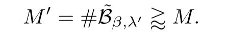

From the de finitions of

λ

and

γ

,we have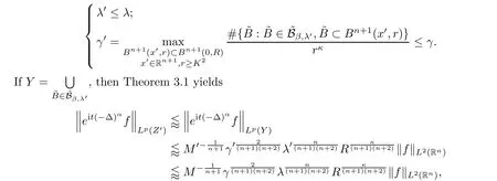

which is the desired(3.6).

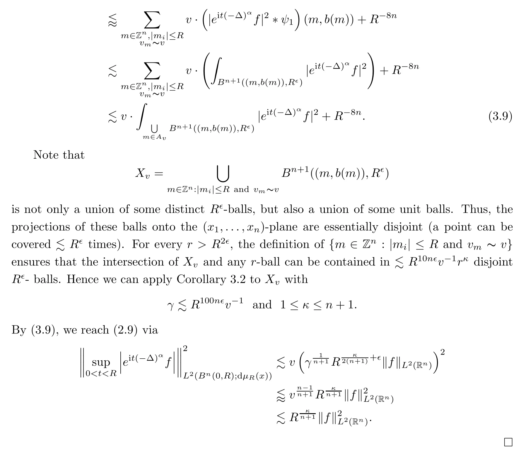
3.2 Proof of Theorem 2.2

In this section,we use Corollary 3.2 to prove Theorem 2.2.

We have

which decays rapidly,then for any(

x,t

)∈R,

denotes the center of the unit lattice cube containing(

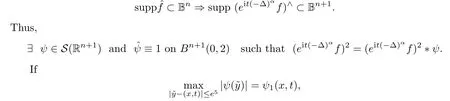
x,t

),and hence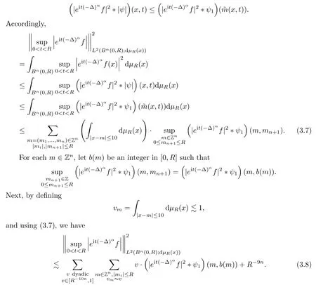

By pigeonholing,we getthat for any small

∊>

0,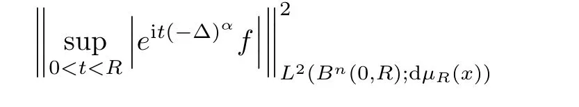

4 Conclusion

4.1 Proof of Theorem 3.1-R≾1

In what follows,we always assume that

Nevertheless,estimate(3.2)under

R

≾1 is trivial.In fact,from the assumptions of Theorem 3.1,we see that

Furthermore,by the short-time Strichartz estimate(see[26,27]),we get that

thereby verifying Theorem 3.1 for

R

≾1.

4.2 Proof of Theorem 3.1-R≫1

First,we decompose the unit ball in the frequency space into disjoint

K

-cubes

τ

.Write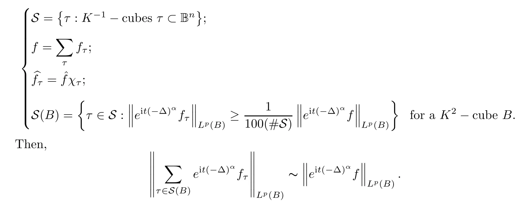

Second,we recall the de finitions of narrow cubes and broad cubes.

We say that a

K

-cube

B

is narrow if there is an

n

-dimensional subspace

V

such that for all

τ

∈S(

B

),

where

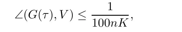
G

(

τ

)⊂Sis a spherical cap of radius∼

K

given by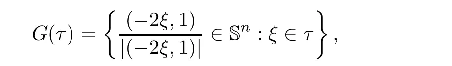

and∠(

G

(

τ

)

,V

)denotes the smallest angle between any non-zero vector

v

∈

V

and

v

∈

G

(

τ

).Otherwise,we say that the

K

-cube

B

is broad.In other words,a cube being broad means that the tiles

τ

∈S(

B

)are so separated that the norm vectors of the corresponding spherical caps cannot be in an

n

-dimensional subspace;more precisely,for any broad

B

,

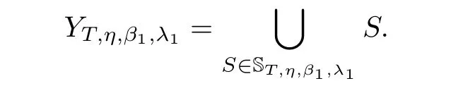
Third,with the setting

we will handle

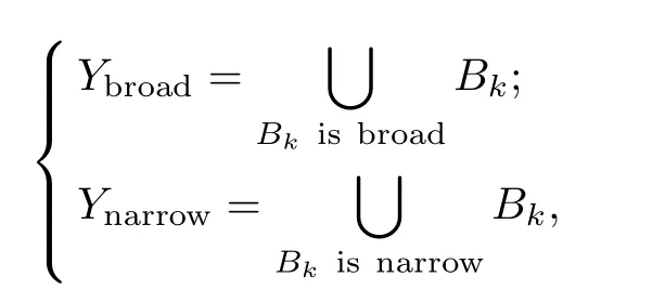
Y

according to the sizes of

Y

and

Y

.Thus,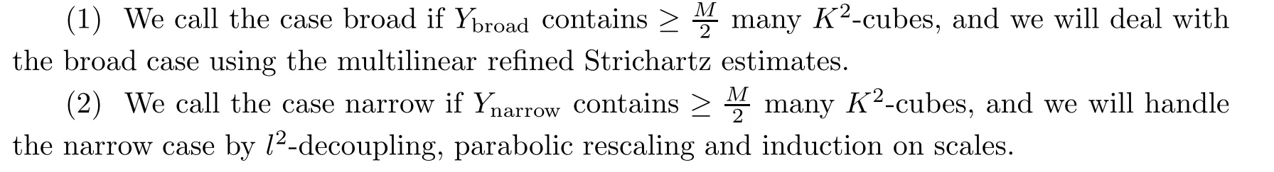

4.2.1 The broad case

Let 0

<c

≪1 and

L

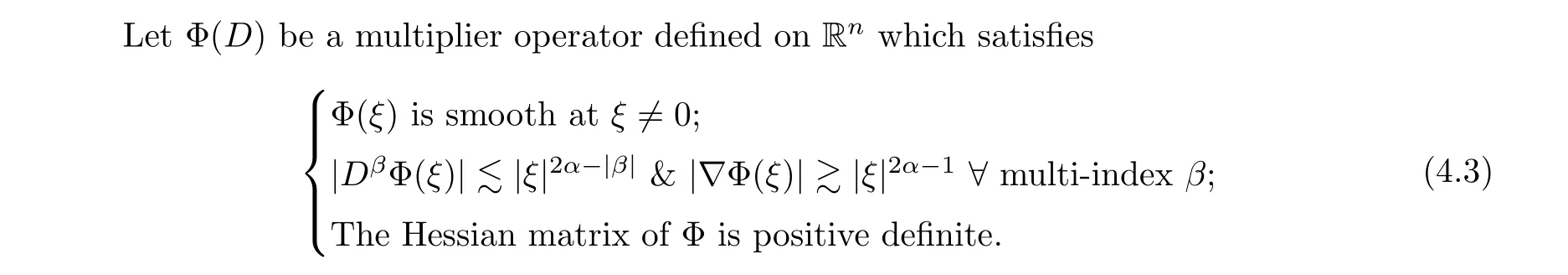
∈N be sufficiently large.We consider a collection of the normalized phase functions as follows: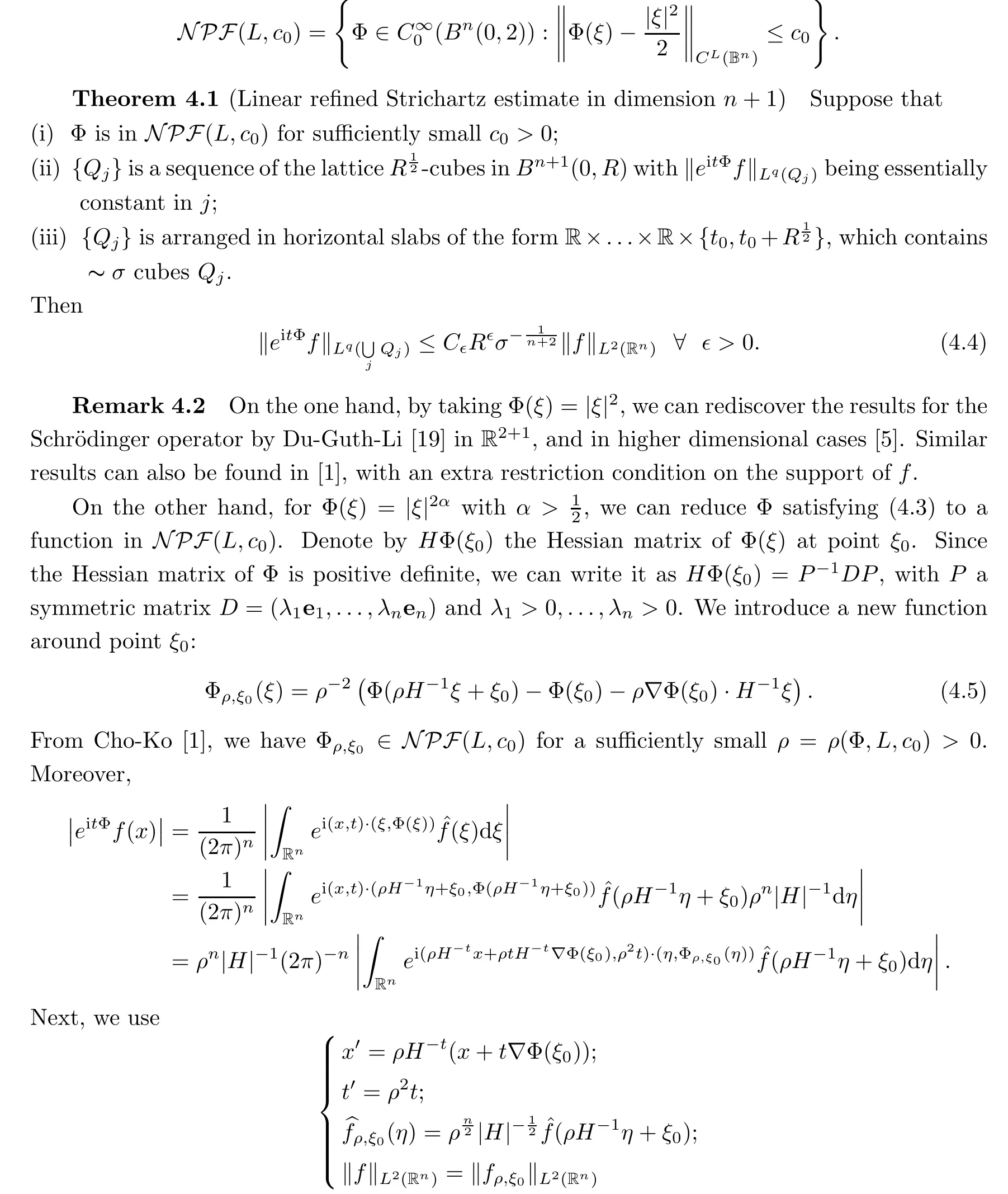

Next we begin the proof of Theorem 4.1.

Proof

We prove a linear re fined Strichartz estimate in dimension

n

+1 by four steps.

and we have that the functions

f

are approximately orthogonal,thereby giving us

By computation,we have that the restriction of

e

f

(

x

)to

B

(0

,R

)is essentially supported on a tube

T

,which is de fined as follows:

Here

c

(

θ

)&

c

(

D

)denote the centers of

θ

and

D

,respectively.Therefore,by a decoupling theorem,we have that

In fact,as in Remark 4.2,we get that

thereby giving us that,if

f

=

f

,

(thanks to|

H

|∼1)

,

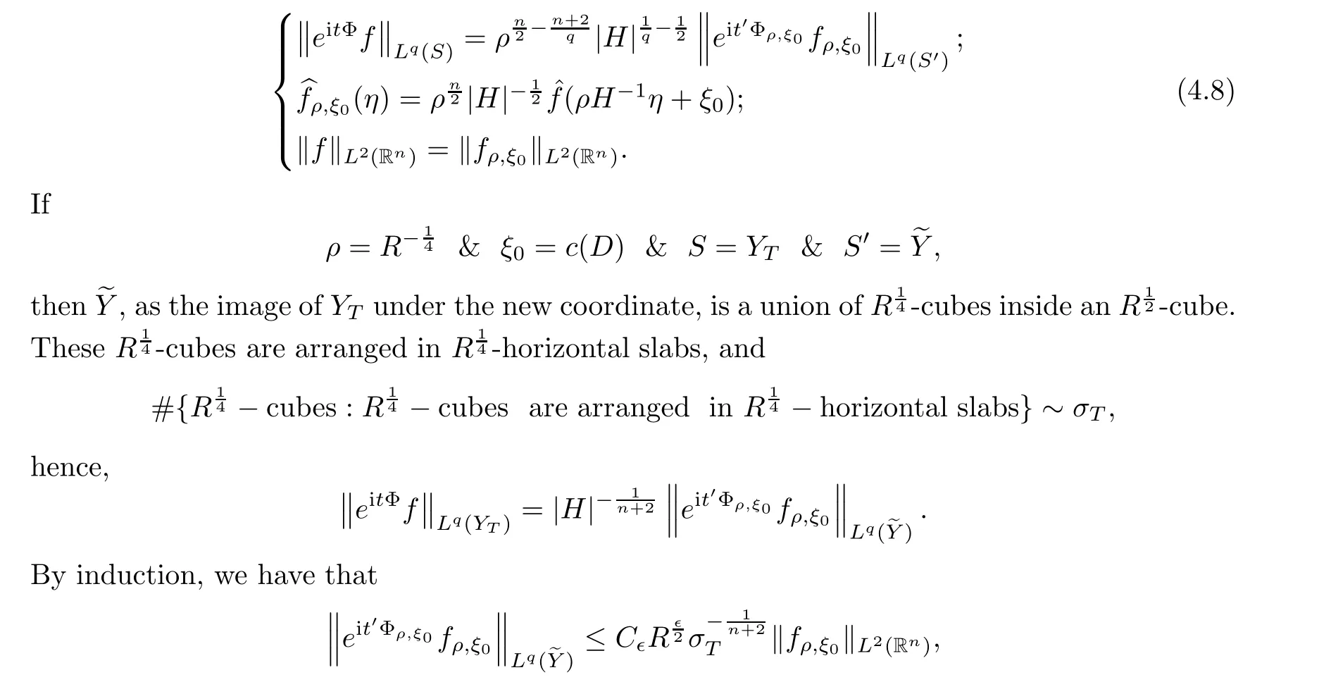
namely that,(4.7)holds.Third,we shall choose an appropriate

Y

.For each

T

,we classify tubes in

T

in the following ways:

Next,we choose the tubes

Y

according to the dyadic size of‖

f

‖.We can restrict matters to

O

(log

R

)choices of this dyadic size,so we can choose a set of

T

’s with T such that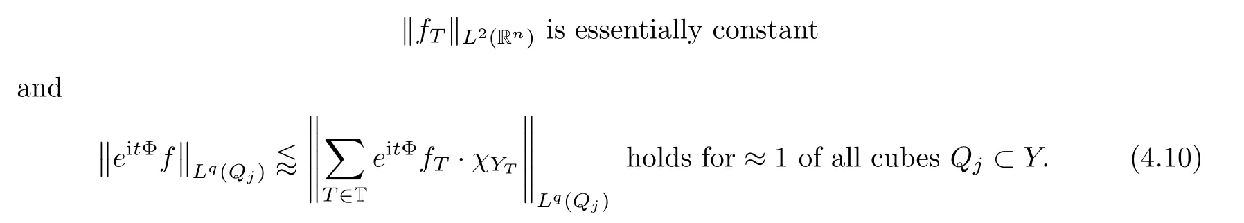

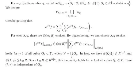
Lastly,we choose the cubes

Q

⊂

Y

according to the number of

Y

that contain them.Denote that

Because(4.10)holds for≈1 cubes and

ν

are dyadic numbers,we can use(4.9)to get

thereby finding that

Fourth,we combine all of our ingredients and finish our proof of Theorem 4.1.

By making a sum over

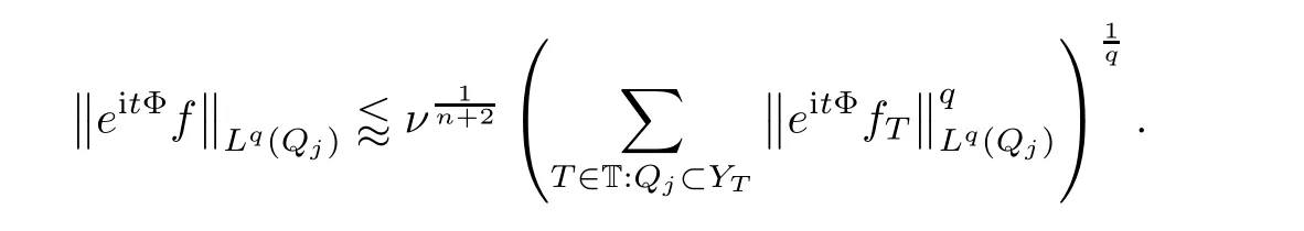
Q

⊂

Y

and using our inductive hypothesis at scale

R

2,we obtain that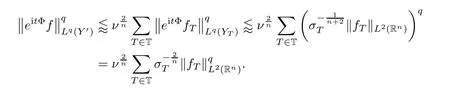

For each

Q

⊂

Y

,since

we get that

thereby utilizing(4.11)and the fact that‖

f

‖is essentially constant among all

T

∈T to derive that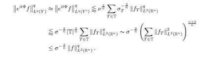

Taking the

q

-th root in the last estimation produces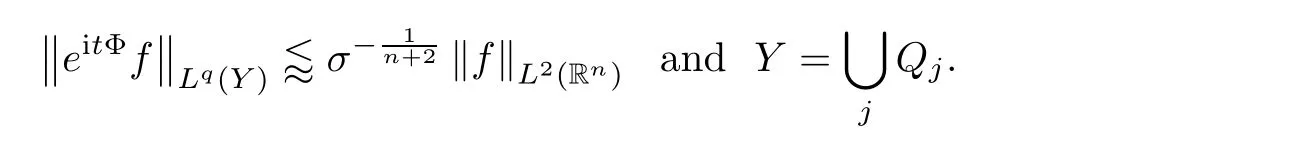

Moreover,Theorem 4.1 can be extended to the following form,which can be veri fied by[22]and Theorem 4.1:

Theorem 4.4

(Multilinear re fined Strichartz estimate in dimension

n

+1.)For 2≤

k

≤

n

+1 and 1≤

i

≤

k

,let

f

:R→C have frequencies

k

-transversely supported in B,that is,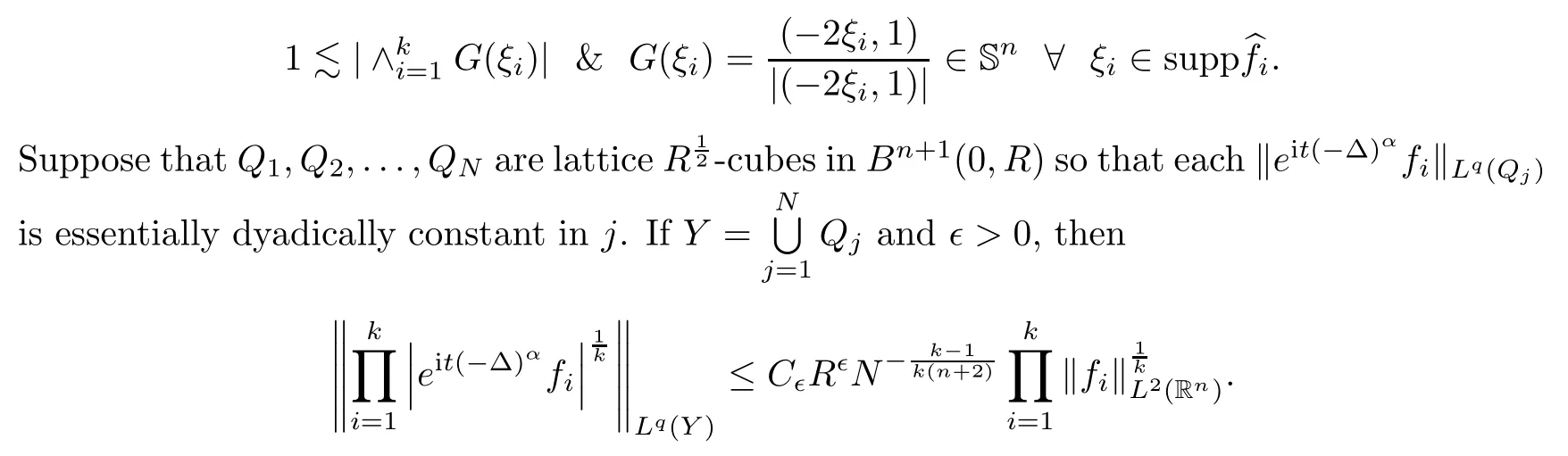

Next,we prove the broad case of Theorem 3.1.

Then,for each

B

∈

Y

,

In order to exploit the transversality and to make good use of the locally constant property,we break

B

into small balls as follows: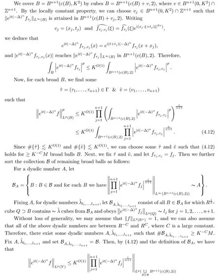

However,the second equivalent inequality of(4.14)follows from de finition(3.1)of

γ

,which ensures that

M

≤

γR

and

γ

≥

K

.

4.2.2 The narrow case

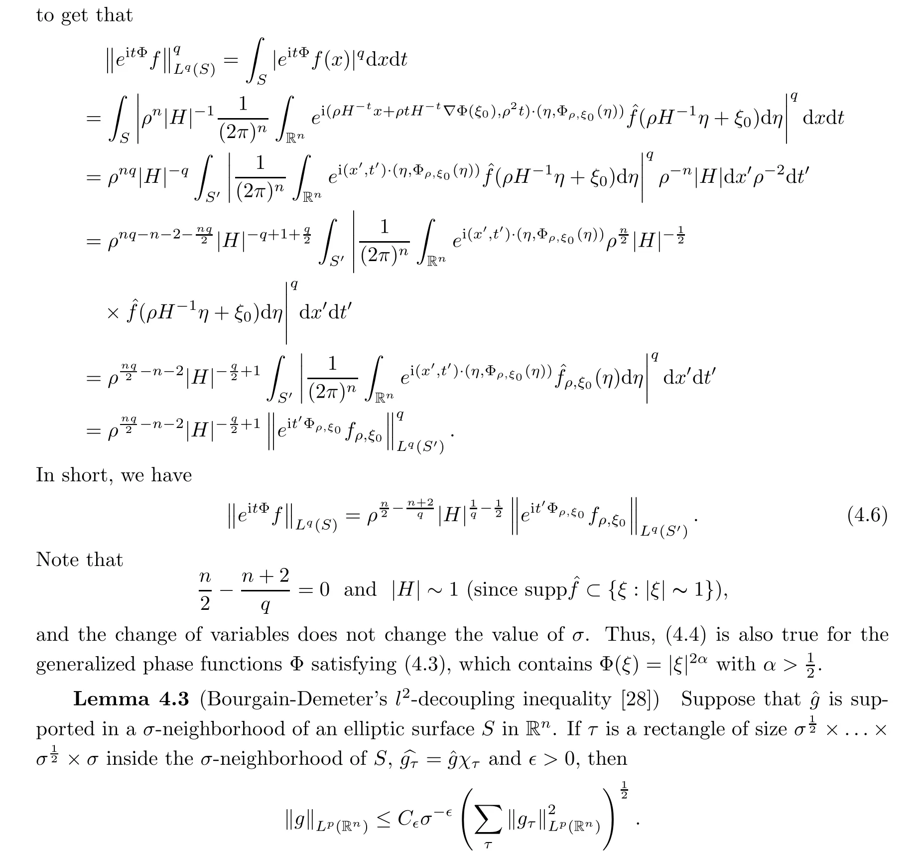
In order to prove the narrow case of Theorem 3.1,we have the following lemma,which is essentially contained in Bourgain-Demeter[28]:

Lemma 4.5

Suppose that(i)

B

is a narrow

K

-cube in Rthat takes

c

(

B

)as its center;(ii)S denotes the set of

K

-cubes which tile B;(iii)

ω

is a weight function which is essentially a characteristic function on

B

;more precisely,that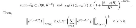

Next,we prove the narrow case of Theorem 3.1.

Proof

The main method we use is the parabolic rescaling and induction on the radius.We prove the narrow case step by step.

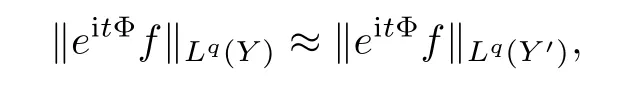
Fourth,let

Then,for

Y

,we can write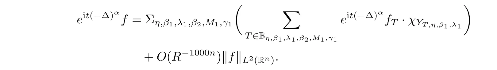

The error term

O

(

R

)‖

f

‖can be neglected.In particular,on each narrow

B

,we have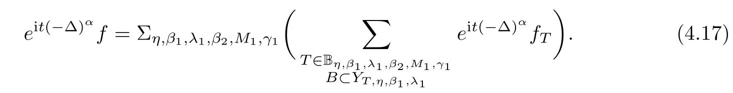

Without loss of generality,we assume that

Therefore,there are only

O

(log

R

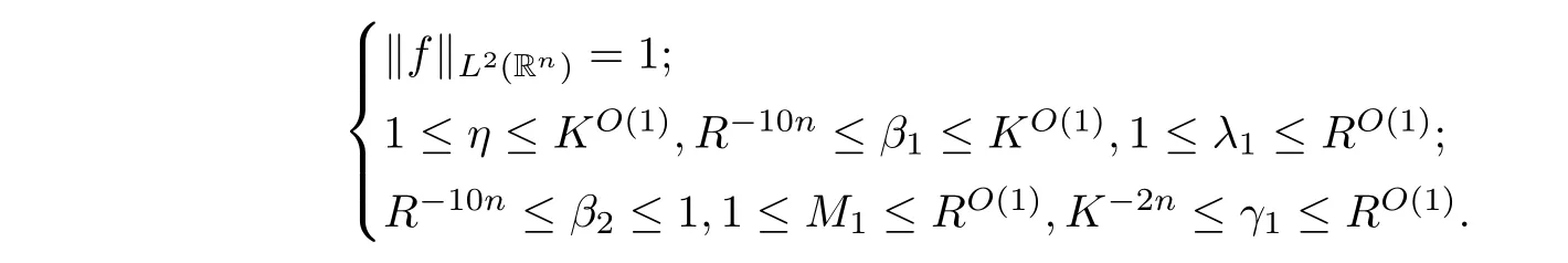
)signi ficant choices for each dyadic number.By(4.17),the pigeonholing,and(4.15),we can choose

η,β

,λ

,β

,M

,γ

such that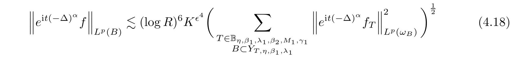

holds for≿(log

R

)narrow

K

-cubes

B

.Fifth,we fix

η,β

,λ

,β

,M

,γ

for the rest of the proof.Let

Let

Y

⊂

Y

be a union of narrow

K

-cubes

B

each of which obeys(4.18)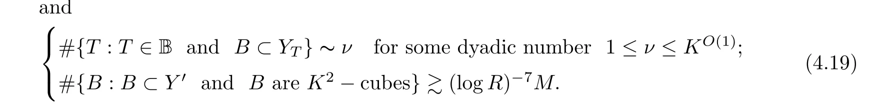

By our assumption that‖

e

f

‖is essentially constant in

k

=1

,

2

,...,M

,in the narrow case,we have that

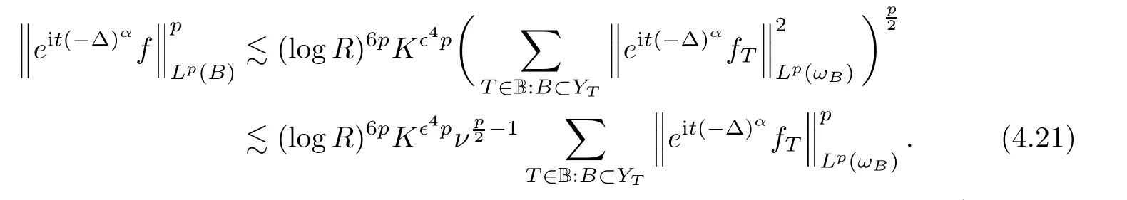
By(4.20)and(4.21),we have

Sixth,regarding each‖

e

f

‖,we apply parabolic rescaling and induction on the radius.For each

K

-cube

τ

=

τ

in B,we write

ξ

=

ξ

+

K

η

∈

τ

,where

ξ

=

c

(

τ

).In a fashion similar to the argument in(4.6),we also consider a collection of the normalized phase functions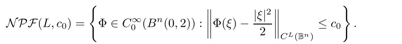

By a similar parabolic rescaling,

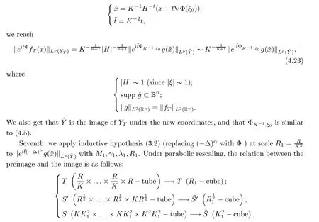
More precisely,we have that

Hence,by the inductive hypothesis(3.2)(replacing(−∆)with Φ)at scale

R

,we have that

By(4.23)and‖

g

‖=‖

f

‖,we get that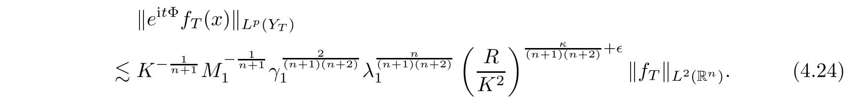

Since(4.24)also holds whenever one replaces Φ with(−∆),we get that

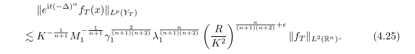
By(4.22)and(4.25),we obtain that

where the third inequality follows from the assumption that‖

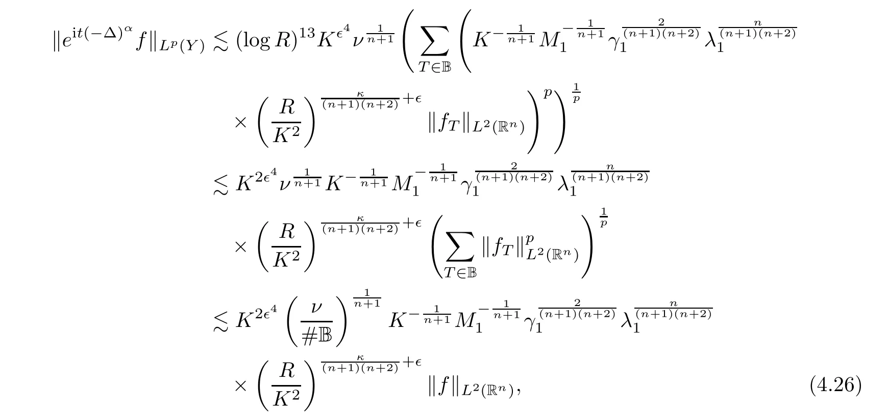
f

‖is essentially constant in

T

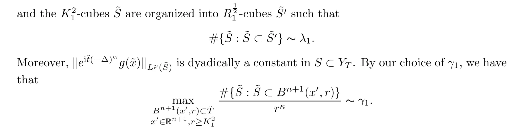
∈B,and then implies that

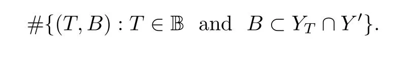
Eighth,we consider the lower bound and the upper bound of

On the one hand,by the de finition of

ν

in(4.19),there is a lower bound

On the other hand,byurchoices of

M

and

η

,for each

T

∈B,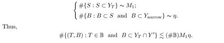

Therefore,we get

Ninth,we want to obtain the relation between

γ

and

γ

.By our choices of

γ

,as in(4.16)and

η

,we get that

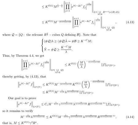
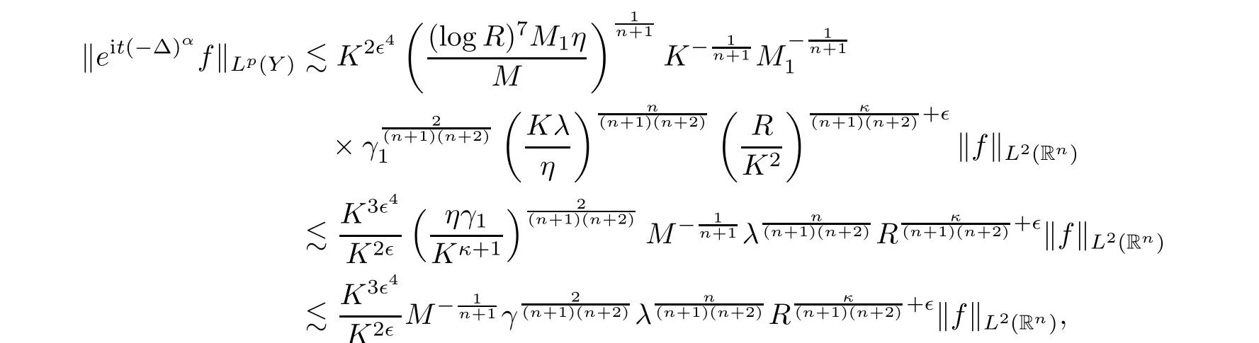
Tenth,we complete the proof of Theorem 3.1.

On the one hand,

Thus it follows that

Inserting(4.27),(4.29)and(4.28)into(4.26)gives that