A novel fault section locating method based on distance matching degree in distribution network

Zhenxing Li,Jialing Wan*,Pengfei Wang,Hanli Weng and Zhenhua Li

Abstract Fault section location of a single-phase grounding fault is affected by the neutral grounding mode of the system,transition resistance, and the blind zone.A fault section locating method based on an amplitude feature and an intelligent distance algorithm is proposed to eliminate the influence of the above factors.By analyzing and comparing the amplitude characteristics of the zero-sequence current transient components at both ends of the healthy section and the faulty section, a distance algorithm with strong abnormal data immune capability is introduced in this paper.The matching degree of the amplitude characteristics at both ends of the feeder section are used as the criterion and by comparing with the set threshold,the faulty section is effectively determined.Finally, simulations using Matlab/Simulink and PSCAD/EMTDC show that the proposed section locating method can locate the faulty section accurately, and is not affected by grounding mode,grounding resistance, or the blind zone.

Keywords: Distribution network, Section location, Intelligent distance algorithm, Wavelet decomposition and reconstruction, Matching degree

1 Introduction

Improving intelligence level [1] and enhancing power supply reliability are some of the development foci in distribution networks.The wiring mode of a distribution network adopts an ungrounded neutral point or grounded neutral point via an arc suppression coil.Because single-phase earth faults account for 80% of all failures [2], research on the locating method of this type of fault has become a hotspot.When a single-phase grounding fault occurs in a distribution system with an arc suppression coil, the zero-sequence current of the fault section tends to be the same as the healthy sections[3], making conventional fault section locating methods difficult to apply.Therefore, it is necessary to propose a new method.

[4–8] realize fault location using line mode head information, but the accuracy of the traveling wave method is not high because of the interference of the branch line in the distribution network [9–11].propose the use of wavelet transform, proxy algorithm and other analysis tools, and the characteristics of the transient information are obtained to achieve fault location by comparison[12–15].propose a fault section locating method based on a linear correlation method using the differences of fault transient zero sequence current at two ends of the fault point.The Pearson correlation coefficient is used to measure the similarity of the transient zero sequence current waveforms at two detection points, and the fault location is realized.

Among the existing fault section locating methods, the linear correlation method has the best location effect.However, this method is greatly affected by grounding resistance and has blind spots.A novel fault section locating method based on the Hausdorff distance algorithm is proposed in [16] and is applied to image processing to measure the similarity between graphics.This algorithm considers the overall feature difference of images while discarding the detailed features between images.The image feature matching function of the Hausdorff distance algorithm uses the zero-sequence current waveform information more comprehensively,so the fault section location based on this algorithm can be more accurate than other methods.

Relying on the faulty feeder, this method uses wavelet decomposition to extract the high-frequency coefficients and reconstructs the zero-sequence current transient components.The transient components at both ends of the section are normalized and the translated data information is used in the Hausdorff distance algorithm after the translation of a data window, and then is traversed to obtain the minimum distance value H.This step can eliminate the influence of asynchronous data on measurement accuracy.The distance value is used to determine the matching degree HS and by comparing the matching degree with the set threshold, the faulty section can be effectively determined.The method can locate the faulty section accurately under different neutral grounding modes and different grounding resistances,while it is also valid in the blind zones of the linear correlation method.

2 Transient characteristics analysis of zerosequence current

2.1 Distribution network equivalent model

To facilitate the analysis, centralized parameters are used.The equivalent circuit of a zero-sequence distribution network in single-phase grounding fault is shown in Fig.1.In developing the equivalent zero-mode network,the accuracy of the equivalence between the fault point and feeder bus is the key to the correctness of the transient characteristics.

In Fig.1, C0bC0nand C0lare the equivalent capacitances of the upstream line of the fault point, the sound feeder, and the downstream line, respectively.L0band L0lare the equivalent inductances of the fault point to the bus and the downstream, respectively.R0band R0lare the resistances of the upstream and downstream,respectively.

According to Fig.1 and [13–15], the instantaneous value of the zero-sequence current transient components of the upstream and downstream are:

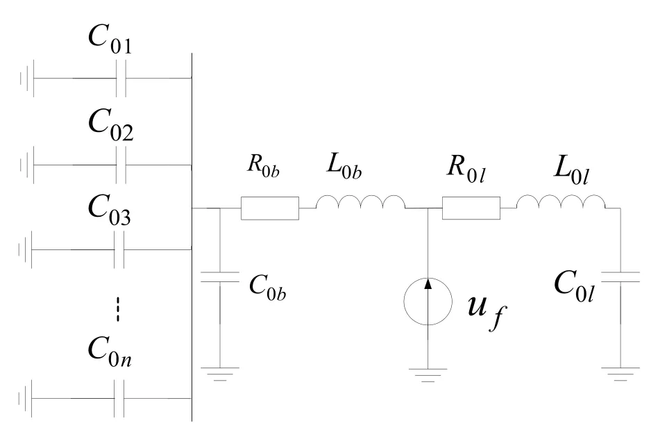
Fig.1 Equivalent circuit of zero-sequence network

where Umis the peak of system phase voltage, φ is the initial fault phase angle.The subscript x indicates the up(b) or down (l) stream.The related parameters and expressions are given in the table below.

Parameter Expression ωx(oscillation frequency) ffiffiffiffiffiffiffiffi 1 L0xC0x q(2)I0 mx (Amplitude)UmωC0x pffiffiffiffiffiffiffiffiffiffiffiffiffiffiffiffiffiffiffiffiffiffiffiffiffiffi ð ωxω sinφÞ2þ cos2 φ(3)αx(Initial phase angle) arctanð ω ωx tanφÞ(4)δx (Attenuation coefficient)R0x 2L0x (5)

2.2 Analysis of amplitude characteristics of zero-sequence current transient components

The difference of the transient currents at the two ends of healthy section in the faulty feeder is only the capacitive current of the section.The amplitudes of the transient currents at both ends are close and the waveforms are also similar.The frequency of the zerosequence current transient component at the upstream of the fault point is mainly determined by the capacitance parameter of the upstream line of the fault point and the healthy feeder.The downstream node is mainly determined by the capacitance parameter of the downstream line of the fault point.As the parameters of the upstream and downstream are quite different, the amplitudes of the transient components of the upstream and downstream nodes are inevitably different, as will be further shown in Fig.2.

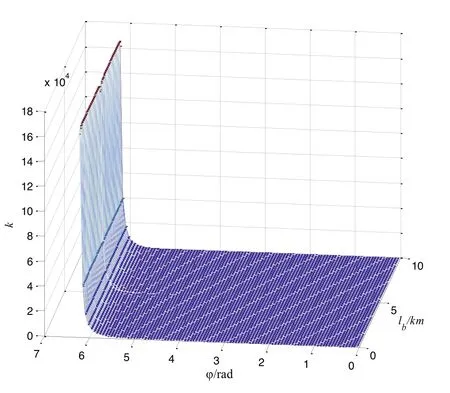
Fig.2 Three-dimensional surface map of amplitude ratio

From (3), the amplitude and amplitude ratio of the transient components at the two ends of the faulty section are:

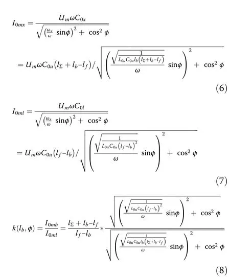
where L0uis the zero-mode inductance of unit length line and C0uis the distributed capacitance to ground.lbis the line length from the fault point to the exit of the bus, and lfis the length of the entire feeder of the fault line.lΣis the sum of all outlet lengths of the system.I0mland I0mbare the amplitudes of the transient components downstream and upstream of the fault point, respectively.k is the amplitude ratio of the transient components at the two ends of the faulty section.

To obtain the general characteristics of the amplitude ratio, its three-dimensional surface map is shown in Fig.2.The value of amplitude ratio is shown in Table 1.When the distance between the fault point and the feeder bus is constant, the amplitude ratio is almost unchanged, while when the initial phase angle is constant,the amplitude ratio is proportional to lb.From Fig.2 and Table 1, it can also be seen that when the fault point is at the exit of the bus and the initial phase angle is π/50,the amplitude ratio k is greater than 1.3.

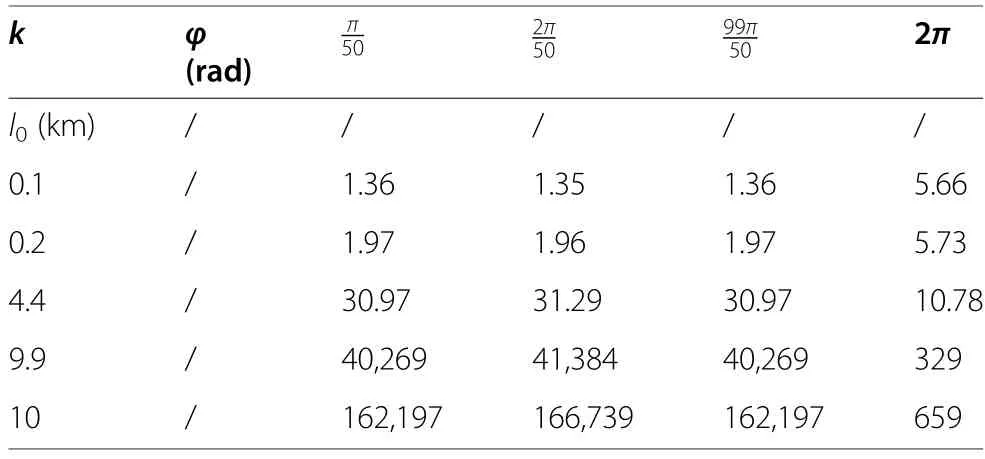
Table 1 The value of amplitude ratio

According to the above analysis, it can be concluded that the amplitude difference of the zero-sequence current transient components at the two ends of the healthy section is small, while the two ends have high similarity in waveforms [17, 18].In contrast, the amplitudes of the zero-sequence current transient components at the two ends of the fault point are significantly different.

2.3 Analysis of influencing factors of the correlation coefficient method

At present, the correlation coefficient method is in the mainstream of fault location methods.According to[13], the location criterion of the correlation coefficient method will fail at special fault points (transient current oscillation frequency of the two ends are similar).Combined with phase, frequency, and attenuation coefficient characteristics, if the transient component frequencies at the two ends of the faulty section are equal (ωb=ωl), the distance from the fault point to the bus lf'can be obtained using (2), as shown as:

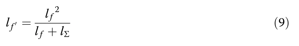
It can be deduced from (9) that there is a set of fault points F' in any feeder line of the distribution network,including the’point and its nearby area.The transient current frequencies at the two ends of the set F' are similar, whileThat is, the set is located in the upstream section of the feeder line.

When a fault occurs, according to (4) and (5), there are:

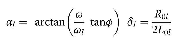
When the fault point is in the set F',thereare:

The phases, frequencies and attenuation coefficients of the zero-sequence current transient components at the two ends of the faulty point set F' are approximately equal.Thus the correlation coefficient of the faulty section is relatively high, and the criterion of the correlation coefficient method will fail to work.The simulation results of the correlation coefficient method will be shown in Table 3 in Section 6.1 to verify the existence of the blind zone.

The timing error, initial fault current angle, data window length and grounding resistance of the wave recording terminal can also influence the correlation coefficient.For the timing error, the correlation coefficient method has a feasible way to solve it [15].Combined with the simulation model and parameters in Section 6, the attenuation performance of the transient component amplitudes under different transition resistances are shown in Table 2.

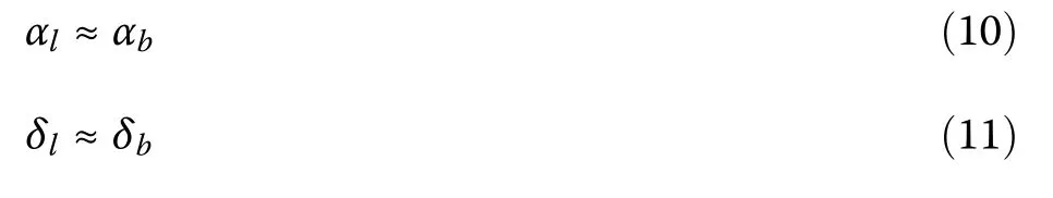
From Table 2, the characteristics of the transient attenuation process are as follows.With the increase in transition resistance, the transient component attenuation rate increases and a weak signal with small amplitude in the data window increases as shown in Fig.3.The existence of a blind zone makes the correlation coefficient higher.When the fault occurs at a different time, the initial fault current angle is different,so the transient current information also changes.

Fig.3 transient attenuation process

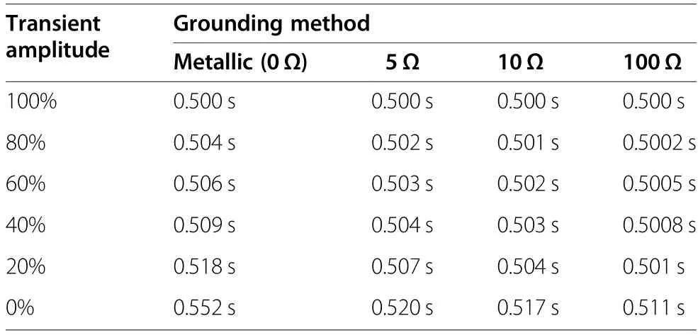
Table 2 Transient attenuation process

According to the above analysis, the initial fault current angle and transition resistance affect the attenuation rate of the transient component.This can lead to the failure of the correlation coefficient method.Therefore, it is necessary to adapt to the special amplitude characteristics and avoid the influence of the above factors.

3 Matching degree principle and optimization scheme

3.1 Acquisition of zero-sequence current transient components

The accurate extraction of zero-sequence current transient components is the premise of the matching degree principle.Wavelet transform can analyze local characteristics in the time and frequency domains at the same time, and use the expansion and translation of the wavelet base to adjust the analysis window adaptively.These characteristics show that the method is suitable for transient information analysis and can be applied to the decomposition analysis of a zero-sequence transient current.

Deriving from [19, 20], this paper designs a wavelet decomposition layer and function by considering sampling frequency and wavelet decomposition characteristics.Wavelet decomposition is used to process the fault transient information and extract the high frequency coefficients after wavelet decomposition,and the transient component is reconstructed using the high frequency coefficients.

3.2 Basic principles of distance algorithm

The matching function of image features is used to measure the waveform distance H, which is calculated as[16]:

where.

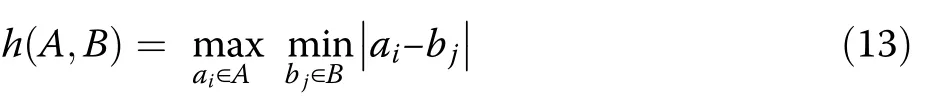
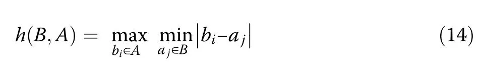
A and B are the set of electrical sampling points with a1, a2, a3, L, an∈A and b1, b2, b3, L , bn∈B.|ai−bj|and |bi−aj| are the distance norms between point sets A and B in(13) and (14), respectively.For any points aq∈A or bq∈B in A or B, |aq−bj| and |bq−aj| are calculated in turn and then the minimum ofis obtained.Considering q=1, 2, 3, L,n, many minimum distance values can be obtained in turn, and then the maximum of these minimum values can be calculated according to (13) and (14).The maximum value is the one-way Hausdorff distance h(A,B) and h(B,A), while the Hausdorff distance h(A,B) can be obtained by(12).

The schematic diagram of the Hausdorff distance algorithm is shown in Fig.4.

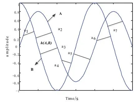
Fig.4 The schematic diagram of the Hausdorff distance algorithm

According to the calculation principle, the Hausdorff distance algorithm is not affected by the weak signal mentioned above.The algorithm can measure the amplitude difference between the two waveforms and find a new angle of the amplitude feature to avoid the blind zone.

3.3 Transient information normalization and locating criterion threshold setting based on the distance algorithm

The data source of the Hausdorff distance algorithm is the zero-sequence current transient components extracted using the wavelet transform.The distance H is calculated by the transient components of the zero sequence current at the two ends of the faulty section, and the matching degree value HS (HS=1 −H)is determined to measure the matching degree of the transient component waveforms at the adjacent node.The closer H is to 0, the closer HS is to 1, and the matching degree of the two waveforms is higher.In the converse situation, the matching degree is lower.

In order to facilitate the setting of the criterion threshold and measure the distance value H at the two ends of the section visually, the data in the data window of the transient components are distributed to [0, 1] by normalization.The normalized data of the transient components are put into the Hausdorff distance algorithm, and the distance H of the adjacent node can be calculated according to (12)–(14).The distance value H reflects the overall difference between the two sequences and is proportional to the difference.

The distance value H at the two ends of the healthy section is close to zero.Thus the theoretical matching value of the healthy section can be set to HST=1.The matching degree value HS is used as the basis for setting.As the HS value at the two ends of the healthy section is close to 1, the criterion threshold setting can be based on the theoretical matching value of HST.

The principles of setting are as follows:

where Krelgenerally takes a value between 1.15 and 1.3.Because HST=1 and Krel=1.2 in this paper (Krelcan be adjusted according to the actual project), HSset=0.83 based on (15).

4 The optimization scheme of matching degree

The existing time setting mode of the data acquisition equipment (FTU) has an error of 1～3 ms, so it will affect the accuracy of the criterion and cannot reflect the actual characteristics of the data, according to [13].In order to eliminate the error, one sequence can be fixed and the data window of another sequence can be translated back and forth to obtain a matching degree.For the faulty feeder, the amplitude and frequency differences between the two ends of the healthy section are small, so the waveform matching degree is the highest when data are synchronized.However, the amplitudes of adjacent nodes at the fault point are obviously different.Therefore, the matching degree of synchronized or asynchronized data is less than the threshold.Therefore, it is necessary to ensure the calculation accuracy of the matching degree at the two ends of the healthy section.

Setting the single move step size of the data window to ΔT=1/fs(fsis the system sampling frequency), the moving data width is ±3ms and the maximum value of total moving steps is N′=2×3×10‐3×fs.The switch number and corresponding section number is x, and the switch number of the feeder section is X.The matching degree HSx→x+1(the matching degree of the xthand the (x+1)thsampling points) is:

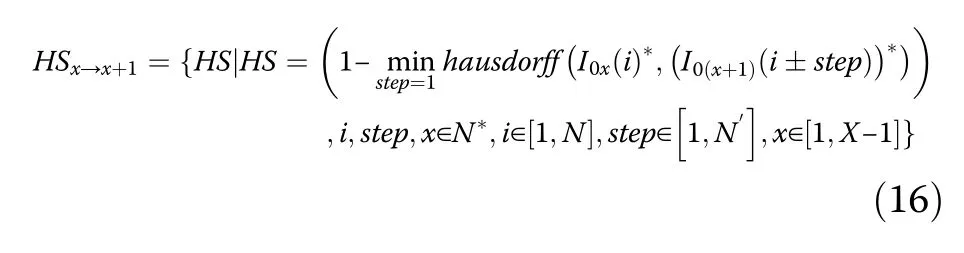
where N is a periodic sampling point in the data window(including the complete transient information after the fault), N′is the movable step, andare the normalized sequence of zero-sequence current transient components of node x and node x+1.

The data window selection principle in the optimization method should consider the actual duration of the transient process to adjust the optimization scheme.The transient process lasts around 1 cycle, and the construction of the matching optimization scheme requires a certain length of data translation step.In order to satisfy the matching optimization scheme, the input data of the Hausdorff distance algorithm can maintain the same number of sampling points N after the data window is moved.The data window needs to have a margin of 2 ∗N′while considering the maximum 3 ms error of time setting mode and fs=10kHz, so the margin can be determined as 100 sampling points and the length of the data window is 1.5 cycles.Thus, 50 sample points are extended to the left and right, respectively, based on the N sampling points.

5 Section locating process

The fault section locating process is shown in Fig.5.

Fig.5 Process of the new section locating method

6 Simulation and discussion

6.1 Results of the correlation coefficient method and distance matching degree method

Matlab/Simulink is used to build a simulation model according to a typical topology of a 35 kV distribution network shown in Fig.6.The system is grounded via an arc suppression coil or ungrounded, and the exit lines are L1-L5.The line lengths and electrical distribution parameters of the lines are:

Fig.6 Multi-feeder distribution network topology

The compensation degree of the arc suppression coil is set to 10%, so Lp=0.81 H.For the simulation model,lf0≈2:6km is calculated according to (9), and it can be determined that the set of F2and its nearby fault points are within the blind zone.

In feeder 2, F1-F5 are the single-phase grounding fault points at different times and under different grounding resistances.The sampling frequency is 10 kHz and the data window is 1.5 cycle.

(a) The linear correlation method

The linear correlation method has the best location performance in section location at present.The linear similarity of the two waveforms is described by the correlation coefficient as:

The results for different grounding resistances (Rg)and fault points (F1 - F5) are shown in Table 3.

(b) The proposed positioning method

Using the positioning method proposed in this paper the results are shown in Tables 4, 5, 6, 7, 8 and 9.Tables 4, 6, 8 are the results with different initial fault current angles and grounding resistances for an ungrounded system, while Tables 5, 7, 9 are the corresponding results for the arc suppression coil grounding system.

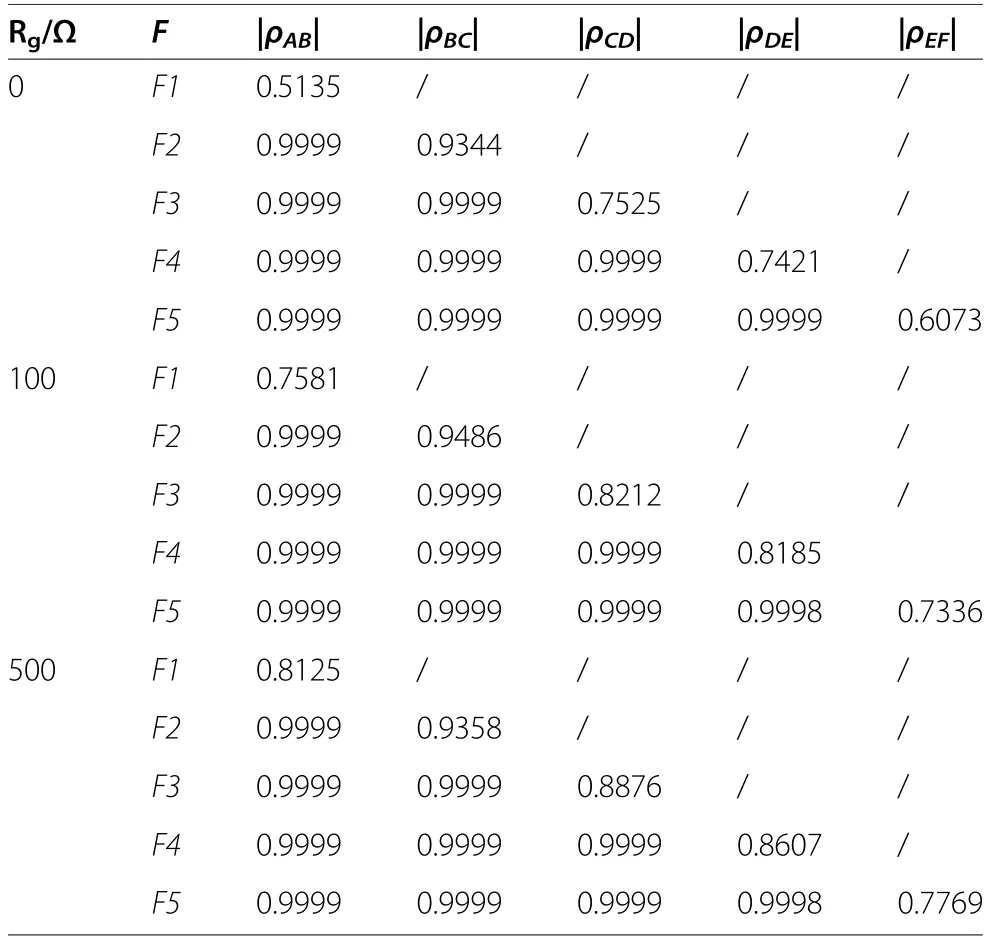
Table 3 Results of the correlation coefficient method(φ=0∘)

Table 4 Results of the proposed positioning method(φ=0∘,ungrounded system)

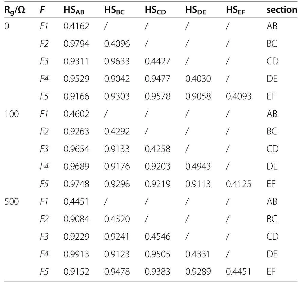
Table 5 Results of the proposed positioning method(φ=0∘, arc suppression coil grounding system)

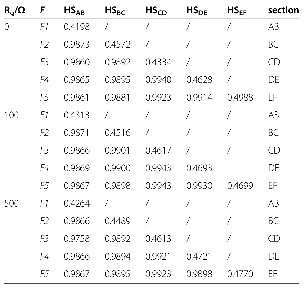
Table 6 Results of the proposed positioning method(φ=30∘,ungrounded system)

Table 7 Results of the proposed positioning method(φ=30∘,arc suppression coil grounding system)

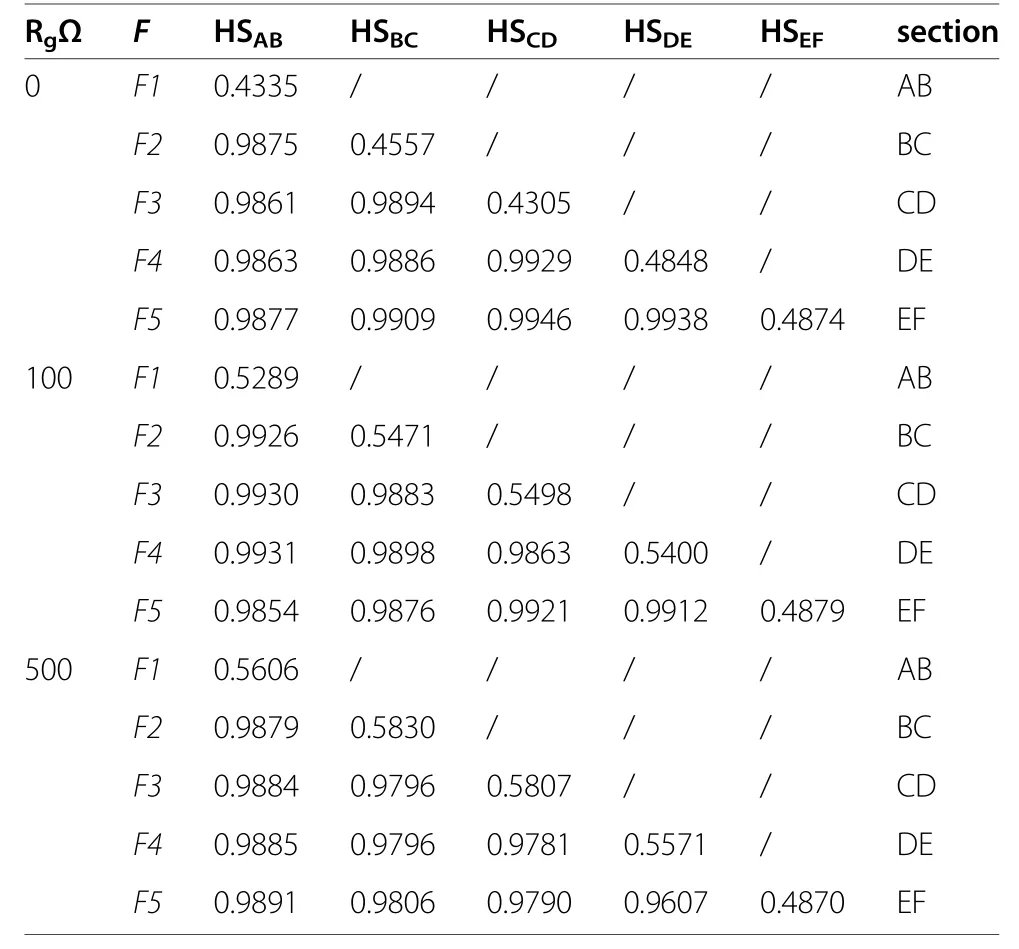
Table 8 Results of the proposed positioning method(φ=60∘,ungrounded system)

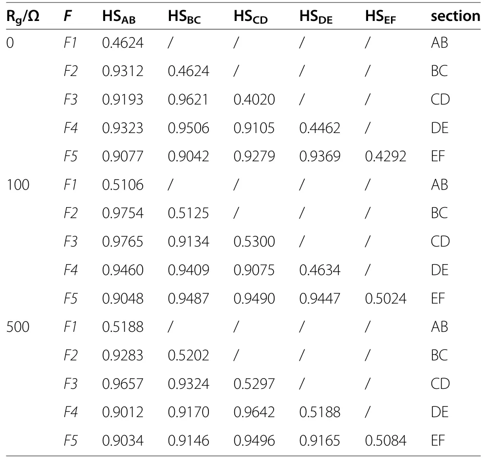
Table 9 Results of the proposed positioning method(φ=60∘,arc suppression coil grounding system)

6.2 Comparison and discussion

The general threshold ρsetis 0.6～0.8.Thus when the correlation coefficient of the two waveforms is greater than the threshold value, it is a healthy section.Otherwise it is a faulty section.In general, the linear correlation method can locate the faulty section, e.g., F1 and F5 can be accurately located.As the grounding resistance increases, the similarity of transient components at the two ends of the fault section become higher, so F2, F3, F4 may be misjudged.When the faultpoint is in the blind zone (section BC), the correlation coefficient at the two ends of the faulty section is high and the faulty section cannot be accurately located.The possibility of misjudgment increases and the accuracy of section location is affected.

It can be concluded that the matching degree method can locate the fault section for different initial fault current angles (0°、30°、60°) and different grounding resistances (0 Ω、100 Ω、500 Ω).The matching degree between the healthy section and the faulty section underdifferent fault conditions is significantly different, so the location is accurate.At the same time, the data window selected by this method is unchanged (the data input to Hausdorff algorithm is a one-cycle wave).The increase of weak current signal in the data window does not affect the calculation results of the Hausdorff algorithm.The fault point F2 on feeder L2 has been analyzed and determined as the fault blind zone.The results showthat the matching degree method is not affected by the fault blind zone.

The section locating method in this paper is not affected by the system grounding mode, the initial fault current angle nor the grounding resistance.Compared with the linear correlation method, the fault section can be located more accurately, and there is no blind zone.In summary, the matching degree method is better thanthe linear correlation method in locating the faulty section.

6.3 IEEE 13-node verification simulation

An IEEE 13-node simulation model is built using PSCA D/EMTDC according to Fig.7.The transformer and overhead lines are set according to standard parameters in the model library.Load parameters are shown in Table 10 and the system is ungrounded.

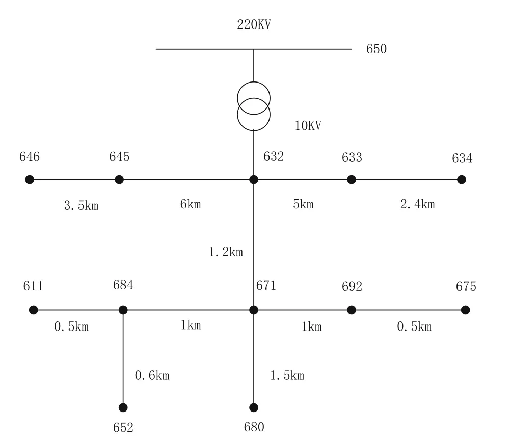
Fig.7 The IEEE 13-node simulation model

For an ungrounded system, the zero-sequence current of the fault line is significantly greater than the healthy section.When faults occur in the sections 632–671 and 671–684, the downstream of the sections will be affected by the branch line capacitance.In Fig.8, I0lis the zerosequence current of the downstream, while I0l1and I0l2are the zero-sequence capacitance current of the branch lines.The downstream zero sequence current of the faulty section increases, and the difference between the upstream and downstream zero sequence current becomes smaller.Because the length of the branch line is short, the impact will not be significant and there are still enough differences at the two ends of the faulty section for positioning.

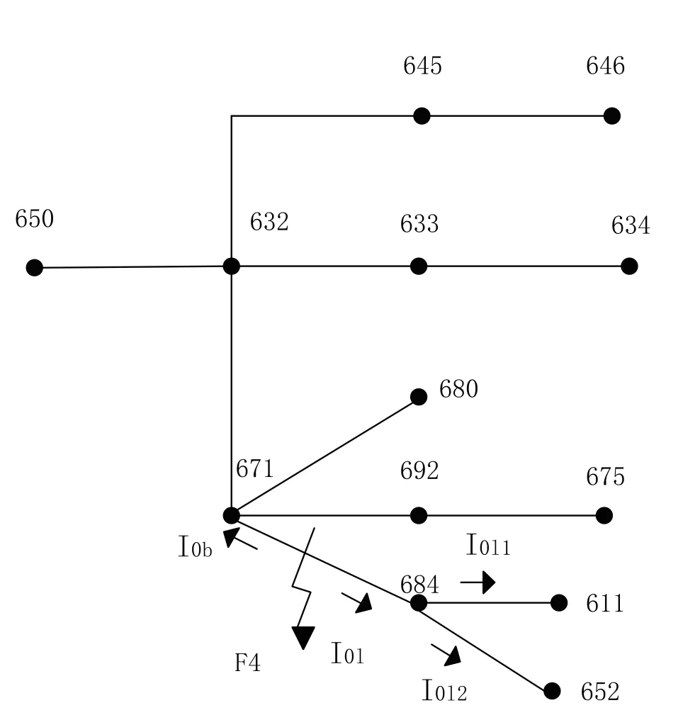
Fig.8 Influence of branch zero sequence capacitance current

F1-F5 are the single-phase grounding fault points under different grounding resistances, and are set in sections 632–671, 671–680, 671–692, 671–684, and 684–611.Based on the faulty section locating process, results of the matching degree method in the IEEE 13-node system are shown in Table 11.The sampling frequency and the data window are the same as the simulation in Section 6.1.

As shown in Table 11, when the downstream of the faulty section is connected with branch lines, the matching degree at the two ends will increase.However,the criterion of the faulty section is still satisfied and all faults in the simulated IEEE 13-node system can be located using the proposed positioning method.

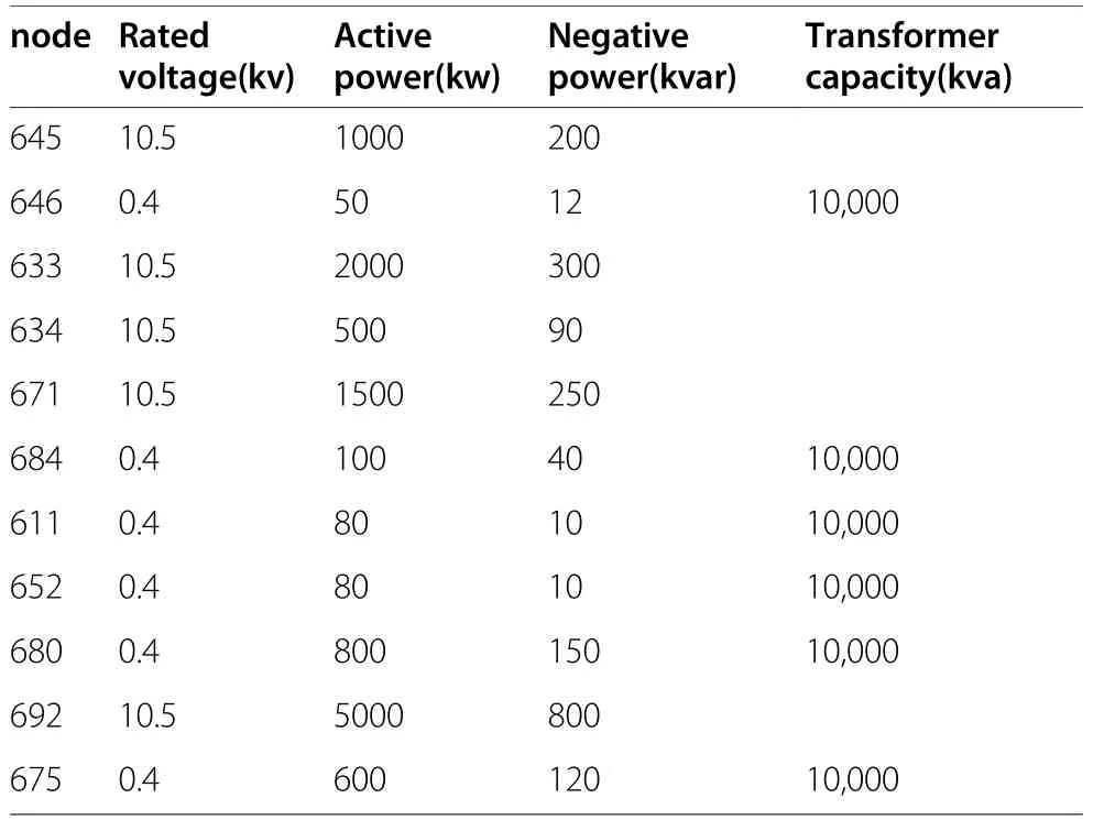
Table 10 Load parameters in the IEEE13 node model

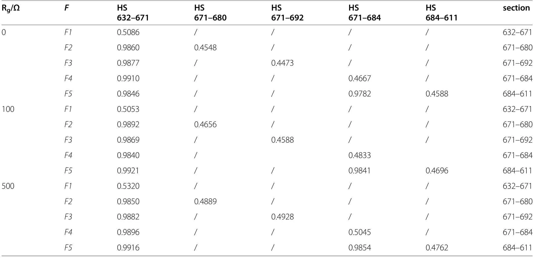
Table 11 Results of the matching degree method in the IEEE 13-node system (φ=0∘)

In summary, the matching degree method can be applied to different models and is not affected by the grounding resistance.

7 Conclusions

In this paper, a novel fault section locating method based on the Hausdorff distance algorithm is proposed.By analyzing the zero-sequence equivalent circuit of the distribution network, the amplitude characteristics of the zero-sequence current transient components are studied,and matching degree is used to determine the faulty section.This method can avoid the influence of data window length, grounding resistance and position blindzone.The simulation shows that the method can accurately detect the faulty section under these influencing factors, thus improving the reliability of fault positioning.

When new energy is connected to the distribution network, the characteristics of the amplitude ratio of adjacent nodes at the point of failure will not be significantly different, and thus, the criterion may fail.Therefore, further research is required on new energy access.

Acknowledgements

Thanks for supporting by the National Natural Science Foundation of China(52077120) and Research Fund for Excellent Dissertation of China Three Gorges University (2021SSPY056).

Authors’ contributions

The amplitude feature and intelligent distance algorithm is used to eliminate the influence of many factors.The author proposes a novel fault section locating method.The author(s) read and approved the final manuscript.

Funding

National Natural Science Foundation of China (52077120)Research Fund for Excellent Dissertation of China Three Gorges University(2021SSPY056).

Availability of data and materials

All data generated or analysed during this study are included in this published article.

Declarations

Competing interests

The authors declare that they have no competing interests.