Self-consistent tomography of temporally correlated errors

Mingxia Huo and Ying Li

1 Beijing Computational Science Research Center,Beijing 100193,China

2 Department of Physics and Beijing Key Laboratory for Magneto-Photoelectrical Composite and Interface Science,School of Mathematics and Physics,University of Science and Technology Beijing,Beijing 100083,China

3 Graduate School of China Academy of Engineering Physics,Beijing 100193,China

Abstract The error model of a quantum computer is essential for optimizing quantum algorithms to minimize the impact of errors using quantum error correction or error mitigation.Noise with temporal correlations,e.g.low-frequency noise and context-dependent noise,is common in quantum computation devices and sometimes even significant.However,conventional tomography methods have not been developed for obtaining an error model describing temporal correlations.In this paper,we propose self-consistent tomography protocols to obtain a model of temporally correlated errors,and we demonstrate that our protocols are efficient for low-frequency noise and context-dependent noise.

Keywords:self-consistent tomography;temporally correlated errors;quantum computer

1.Introduction

How to correct errors is one of the most critical issues in practical quantum computation.In the theory of quantum fault tolerance based on quantum error correction(QEC),an arbitrarily high-fidelity quantum computation can be achieved,providing sub-threshold error rates and sufficient qubits[1].Recently,error rates within or close to the sub-threshold regime have been demonstrated in various platforms[2–6].These error rates are measured using either randomized benchmarking(RB)[7–13]or quantum process tomography(QPT)[14,15].RB only estimates an average effect of the noise,and QPT can provide a model of error channels.Rigorously speaking,whether or not a quantum system is in the sub-threshold regime is not only determined by the error rate but also the detailed error model[16,17],including correlations between errors[18].Therefore,an error model describing correlated errors is important for verifying subthreshold quantum devices.We can also optimize QEC protocols by exploring these correlations[16,19],which is crucial for the early-stage demonstration of small-scale quantum fault tolerance.Given the limited number of qubits and error rate close to the threshold,we need to carefully choose the protocol to observe any advantage of QEC[20–28].

We may still need many years to realise a fault-tolerant quantum computer[29,30],however noisy intermediate-scale quantum(NISQ)computers are likely to be developed in the near future[31–33].Quantum error mitigation is an alternative approach to high-fidelity quantum computation[34–37],which does not require encoding,therefore,is more promising than QEC on NISQ devices.In quantum error mitigation using the error extrapolation,we can increase errors to learn their effect on the observable representing the computation result.Once we know how the observable changes with the level of errors,we can make an extrapolated estimate of the zero-error computation result.This extrapolation can be implemented directly on the final result or each gate using the quasi-probability decomposition formalism.The effect of errors depends on the error model.Therefore,we need to increase errors according to the model of original errors in the system,i.e.at first we need a proper error model of original errors.The error model can be obtained using gate set tomography(GST)[6,38–42],a self-consistent QPT protocol.With the self-consistent error model,the effect of errors on the computation result can be eliminated,under the condition that errors are not correlated[36].However,correlations are common in quantum systems[43–45],e.g.the slow drift of laser frequency can cause time-dependent gate fidelity in ion trap systems[46–50],which limits the fidelity of quantum computation on NISQ devices.Neither RB nor conventional QPT can provide an error model describing temporal correlations[6,10–13].

In this paper,we propose tomography protocols to obtain the model of temporally correlated errors without using any additional operations accessing the environment.Our protocols reconstruct the error model in the self-consistent manner[6,38–42],i.e.the model may be different from the actual one but can fit the experimentally measured data.Temporal correlations are caused by the correlations between the system and the environment.Without a set of informationallycomplete state preparation and measurement operations,we cannot implement conventional QPT on the environment.We find that quantum gates are fully characterized by a set of linear operators acting on a subspace of Hermitian matrices,which can be measured in the experiment only using themselves even without information completeness.However,these operators may not be complete completely positive(CP)maps as in conventional QPT.We term our method as linear operator tomography(LOT),which can be used to reconstruct an operator representation of quantum gates without using additional operations on the environment.A tremendous amount of experimental data may be required to obtain the exact model of temporally correlated errors.For the practical implementation,we aim at an approximate error model,and we find that efficient approximations for low-frequency timedependent noise and context-dependent noise exist[51,52].Practical protocols are proposed and demonstrated numerically.Error rates estimated using RB and GST may exhibit significant difference due to temporal correlations[6].In numerical simulations,we show that RB and LOT results coincide with each other even in the presence of temporal correlations.

The paper is organized as follows.In section 2,we first introduce a general model of a quantum computer including the environment,wherein temporal correlations are caused by the environment.In section 3,we show that in principle by only using operations for operating the system,we can reconstruct a self-consistent model of both the system and the environment.The exact LOT protocol is introduced in section 3.In section 4,we present the condition for performing a truncation on the system-environment(SE)state space.In section 5,we discuss low-frequency time-dependent noise and context-dependent noise.We show that a lowdimensional state space can characterize these two types of temporally correlations.In section 6,we give two approximate tomography protocols for the practical implementation.In section 7,we demonstrate the protocol in numerical simulations.

2.The model of a quantum computer

For illustrating how to describe errors with temporal correlations,we start with an example in ion trap systems.If the quantum gate is driven by the laser field,usually the gate fidelity depends on the laser frequency λ[46–50].The laser frequency drifts with time,and usually we are not aware of its instant value.We use λ to denote a time-dependent random variable,such as the laser frequency.The stochastic process of λ is characterized by the probability distribution(f),i.e.the value of λ at time t is f(t),and(f)is the probability density in the space of functions f(t).We use the superoperatorOS(λ)to denote the gate operation given by the laser frequency λ.With the initial state ρS,the output state after two gatesOSand OS′ at t andt′,respectively,readsWe can find that the statecannot be factorized as two independent operations on the initial state.Therefore,conventional QPT cannot be applied[6,14,15,38–42].

For simplification,we assume that λ changes slowly with time,and the typical time that λ changes is much longer than the time scale of a quantum circuit,i.e.the time from the state preparation to the measurement.In this case,we neglect the change of λ within each run of the quantum circuit,i.e.f(t′)=f(t)for two gates in the same run.We also assume that the distribution is stationary,then the distribution of the instant value,i.e.is time-independent.With the distribution of the instant value,we can rewrite the output state in the form=∫dλ p(λ)OS′(λ)OS(λ)(ρS).

We can factorize multi-gate superoperators by introducing the state space of the laser frequency.We use∣λ∣Eto denote the state corresponding to the laser frequency λ.The state space of∣λ∣Ecan be virtual,i.e.it is not necessary that∣λ∣Ecorresponds to a pure state in a physical Hilbert space.The initial state of qubits and the laser frequency can be expressed asThen the superoperator of a laser-frequency-dependent gate can be expressed aswhere[U]denotes a superoperator[U](ρ)=UρU†.After two gates,the state of the system and the laser frequency readswhich is in the factorized form.One can find that

We note that multi-gate superoperators can be factorized following a similar procedure for noise with any spectrum,i.e.the change of the variable λ in the time scale of a quantum circuit can be nonnegligible or even significant,as we will show in section 5.1.It is straightforward to generalize the approach to the case of multiple random variables,e.g.the gate fidelity depends on a set of drifting laser parameters,and the case that the initial state of the system also depends on random variables.

By introducing the environment,which is the frequency space in the example,we can describe temporally correlated errors.Such a formalism has been used in an ion-trap tomography experiment[6],in which a classical bit is introduced to represent the environment memory.With one classical bit and one qubit,the tomography is implemented on an eightdimensional state space.

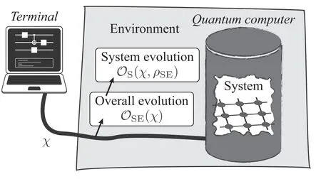
Figure 1.Quantum computer controlled by the state of a terminal.The state of the terminal χ results in the evolutionOSE(χ)of the system and environment.The evolution of the systemOS(χ ,ρSE )depends on both the terminal state χ and the state of the system and environment at the beginning of the evolution ρSE.

Now,we introduce a general model of quantum computer.For a quantum computer with n qubits,we call the 2n-dimensional Hilbert space of qubits the system.Degrees of freedom coupled to the system form the environment,including but not limited to all random variables determining the evolution of the system.Quantum computation is realised by a sequence of quantum gates.The gate sequence is stored in a terminal,e.g.a classical computer,and the evolution of the SE is controlled by the terminal as shown in figure 1.We use χ to denote the state of the terminal indicating‘Implement the gate χ’and superoperatorOSE(χ)to denote the corresponding evolution of SE.Here χ is a deterministic parameter rather than a random variable.By setting χ according to the gate sequence,we realise the quantum computation.We assume that the Born-Markov approximation can be applied to the terminal and SE,and operations on SE are Markovian and factorized.For the gate sequence χ1,χ2,…,χN,the overall evolution of SE isOSE(χN)…OSE(χ2)OSE(χ1).

In this model,the time dependence for operations on the system are not expressed explicitly.Operations on SE are timeindependent.However,corresponding system operations are stochastic and depend on the environment state.When the environment state evolves,which is driven by SE operations,system operations evolves accordingly.In section 5.1,we will give an example that SE operations drive the stochastic process of the environment.In this way,we can describe errors with general temporal correlations,not only correlations caused by classical random variables such as laser frequencies,but also correlations caused by the coupling to a quantum system in the environment.

In general,the evolution of the systemOS(χ,ρSE)depends on not only χ but also the state of SE at the beginning of the evolution ρSE.If the system and environment are correlated in ρSE,the system evolution may not even be CP[53].If the system evolutionOS(χ,ρSE)=OS(χ)does not depend on ρSE,the overall system evolution of a gate sequence isOS(χN)…OS(χ2)OS(χ1).In this case,conventional QPT can be applied,we can obtainOS(χ)up to a similarity transformation using GST[6,38–42],and the computation error can be mitigated as proposed in[36].By introducing the environment,non-Markovian processes can be reconstructed using quantum tomography[54].

From now on,we focus on states and operations of SE and neglect the subscript‘SE’.All states,operations and observables without a subscript(‘SE’,‘S’or‘E’)correspond to SE;and subscripts‘S’and‘E’are used to denote the system and the environment,respectively.

We would like to remark that LOT protocols proposed in this paper cannot reconstruct the complete CP maps acting on SE as in conventional QPT protocols.In LOT,we only use the operations designed to operate the system,i.e.quantum gates for the computation,which actually act on SE because of imperfections.Given the limited accessibility to the environment,it is unrealistic to implement informationallycomplete state preparation and measurement for the full tomography of SE.

2.1.State,measurement,operations and Pauli transfer matrix representation

A quantum computer is characterized by a set of linear operators:the initial state ρinwhich is a normalized positive Hermitian operator,the measurement(i.e.measured observable)Qoutwhich is also a Hermitian operator,and a set of elementary computation operations{O(χ)}which are CP maps.We remark that,ρin,Qoutand{O(χ)}describe the actual quantum computer(including both the system and environment)rather than an ideal quantum computer,and they are all unknown therefore need to be investigated in tomography.The quantum computation is realised by a sequence of elementary operations on the initial state.The set of operation sequencesO={O(χN)…O(χ2)O(χ1) }includes all operations generated by elementary operations{O(χ)}.

We focus on the case that the quantum computer only provides one option of the initial state ρinand one option of the observable to be measured Qout.It is straightforward to generalize our results to the case that multiple options of initial states and observables are available.

In this paper,we use Pauli transfer matrix representation[6,38–42]:∣ρ》is a column vector with elements∣ρ》σ=Tr(σρ);《Q∣is a row vector with elementsthen an quantum operationO can be expressed as a square matrix with elementsHere,σ and τ are Pauli operators or generalized Pauli operators,i.e.Hermitian operators satisfyingTr(στ)=dHδσ,τ,and dHis the dimension of the Hilbert space of SE.All these vectors and matrices are real and-dimensional.For a state ρ and an observable Q,《Q∣ρ》=Tr(Qρ)is the mean of the observable Q in the state ρ.For an operationO,∣O(ρ)》=O∣ρ》is the vector corresponding to the state O(ρ).Therefore,the mean of the observable Q in the state ρ after a sequence of quantum operations readsTr[QON…O2O1(ρ)]=《Q∣ON…O2O1∣ρ》.

3.Self-consistent tomography without information completeness

Information completeness is required by conventional QPT protocols.If we can prepare a complete set of states{∣ρi》=Oi∣ρin》 }and measure a complete set of observableslinearly independent vectors in each set,we can implement QPT on SE to reconstruct the CP maps of quantum gates.Here,the CP maps act on SE.However,information completeness for SE is unrealistic.

In this section,we demonstrate that it is possible to exactly characterize a set of quantum gates using tomography without information completeness.In the LOT formalism,we obtain a set of operators acting on a subspace of Hermitian matrices to represent quantum gates,which may not be complete CP maps without information completeness.Such an operator representation is adequate in the sense that given the initial state,an arbitrary operation sequence and the observable to be measured,the average value of the observable can be computed using these operators.

Because information completeness is not required,we can use LOT to characterize the quantum computer even in the presence of temporal correlations.In this section,the feasibility is not our concern.In the following sections,we will discuss how to adapt the protocol for the purpose of practical implementation.

3.1.Linear operator tomography

With only computation operations,which are designed to operate the system but act on SE because of imperfections,usually we do not have complete state and observable sets,therefore,we cannot access the entire space of Hermitian matrices.

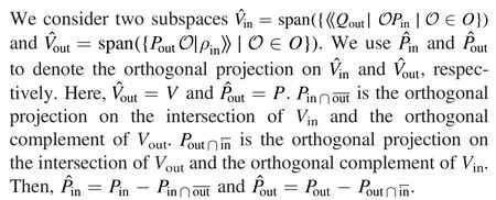
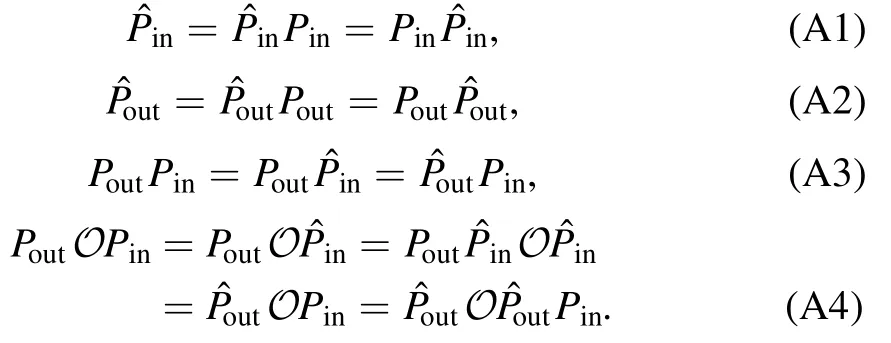
Given an initial state ρin,an observable Qoutand a set of elementary operations{O(χ)},we consider three subspaces of Hermitian matrices as follows.The subspaceVin=span({O∣ρin》∣O∈O})is the span of all states that can be prepared in the quantum computer,and the subspaceVout=span({《Qout∣O ∣O∈O})is the span of all observables that can be effectively measured.Note that O is the set of all operations generated by elementary operations.We use Pinand Poutto denote the orthogonal projections on Vinand Vout,respectively.The third subspace isV=span({PoutO∣ρin》∣O∈O}),and we use P to denote the orthogonal projection on V.

The subspace V is the space of Hermitian matrices that the finite set of operations can access to.If V is the entire Hermitian-matrix space with the dimension,states and observables are complete,then LOT is the same as GST.In general,the completeness is not required in LOT.

Our first result is that in order to fully characterize the quantum computer,we only need to reconstructP∣ρin》,《Qout∣Pand{PO(χ)P} in the tomography.The reason is that,for an arbitrary sequence of operations in O,we have

See appendix A for the proof.We would like to remark that the conclusion is the same for the subspace span({《Qout∣OPin∣O ∈O}).

With this result,we can perform the tomography in a similar way to GST.We note that the protocol presented in this section is for the purpose of illustrating the self-consistent formalism rather than the practical implementation,and we discuss the practical implementation later.We need to assume that the dimension of the subspace V is finite and known,see discussions at the end of this section.The dimension of V isdV=Tr(P).The exact LOT protocol is as follows:

•Choose a set of states{∣ρi》=Oi∣ρin》}and a set of observablesHere,Oi,Ok′∈O,i,k=1,…,d and we take d=dV.We always take∣ρ1》=∣ρin》 and《Q1∣=《Qout∣.

•These states and observables must satisfy the condition that{P∣ρi》 }and{《Qk∣P}are both linearly independent.According to the definition of the subspace V,states and observables satisfying the condition always exist and can be realised in the quantum computer using the combination of elementary operations.

•Obtain matrices g=MoutMinandfor each χ in the experiment.Here,Min=[∣ρ1》…∣ρd》]is the matrix with{∣ρi》 }as columns,andMout=[《Q1∣T…《Qd∣T]Tis the matrix with{《Qk∣}as rows.Each matrix element can be measured in the experiment.The elementgk,i=《Qk∣ρi》is the mean of Qkin the state ρi.The element《Qk∣O(χ)∣ρi》 is the mean ofQkin the state ρiafter the operation O(χ).

•When{P∣ρi》 }and{《Qk∣P}are both linearly independent,g is invertible.We remark that{P∣ρi》}and{《Qk∣P}may not be linearly independent when{∣ρi》}and{《Qk∣}are linearly independent because of the projection P.

for an arbitrary sequence of operations in O.See appendix A for the proof.

•Choose a d-dimensional invertible real matrixand compute

Here,M•,iand Mk,•denote the ithcolumn and the kthrow of the matrix M,respectively.The error model of the quantum computer is formed byandwhich correspond to∣ρ》,《Q∣and{O(χ)},respectively.

According to equation(2),we have

The first line is the computation result according to the error model(the tomography result),and the second line is the experimental result of the actual quantum computer,which are equal.In this sense the error model is exact.The exactness of the error model does not rely on how to choose the matrixIf we choose a different matrixthen we can obtain another error modelandwhereBoth error models can exactly characterize the quantum computer,because the difference between two error models is only asimilarity transformation[6,38–42,55].

If states and observables are informationally complete for SE,V is the entire Hermitian-matrix space of SE,and LOT is the same as GST applied on SE.Without temporal correlations,the states and observables are usually informationally complete for the system,i.e.V is the entire Hermitian-matrix space of the system,and LOT is the same as GST applied on the system.With temporal correlations,in general V is neither the entire space of SE nor the entire space of the system,in which case LOT is different from GST.

The error model reconstructed using LOT can only be applied to states in the subspace Vinand observables in the subspace Vout.If the state is not in Vinor the observable is not in Vout,the error model cannot predict the computation result as in equation(3).This is different from GST,in which the reconstructed model can be applied to any state and observable.

In the exact LOT protocol introduced in this section,we have assumed that the dimension of the subspace V is known.If we can collect all the data generated by the operation set O,we can find out the dimension of V by analyzing the number of linearly independent states(in the subspace Vout).In section 6,we introduce approximate LOT protocols for the practical implementation,in which we do not need to assume that the dimension of V is known.

4.Space dimension truncation

Usually,the environment is a high-dimensional Hilbert space.Although only the subspace V is relevant in the exact LOT,its dimension could still be too high to allow the exact LOT to be implemented.Therefore,a practical LOT protocol is approximate and requires that a low-dimensional subspace approximately characterize the quantum computer.Here,we give a sufficient condition for the existence of such a subspace.

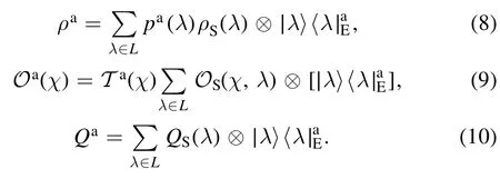
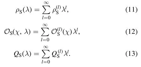
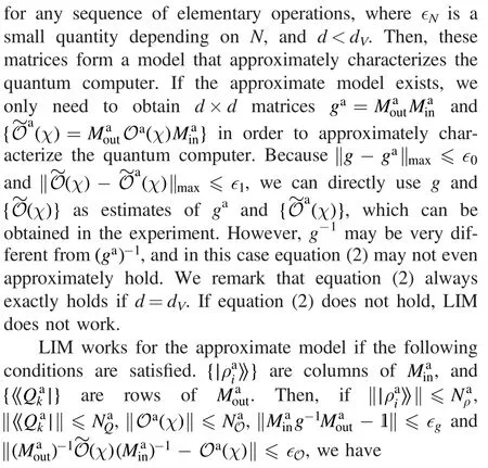
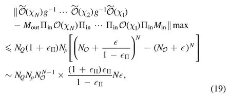
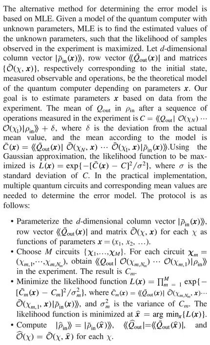
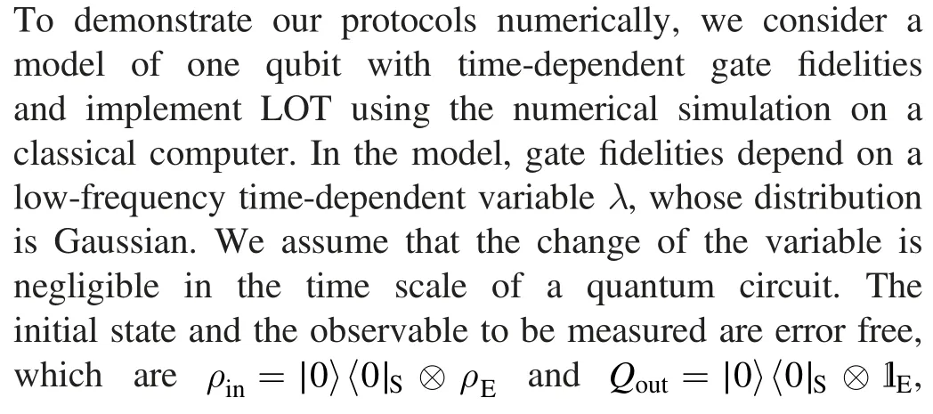
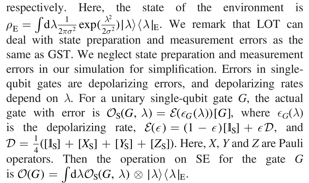
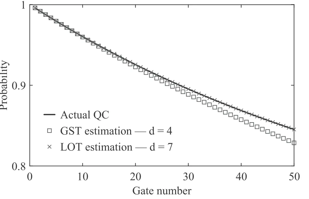
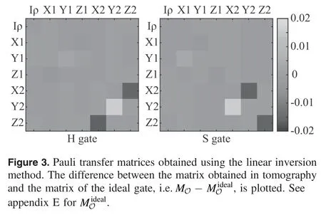
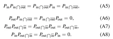
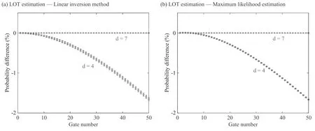
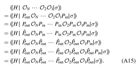
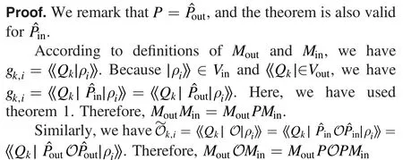
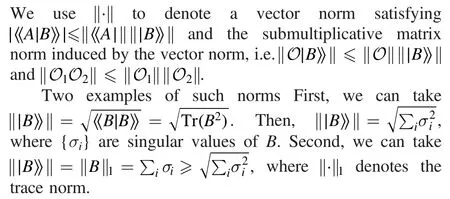
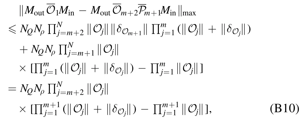
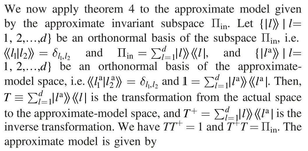
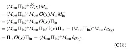
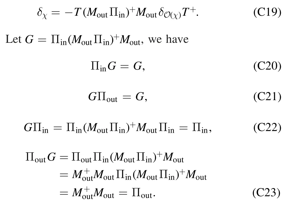
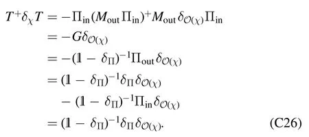
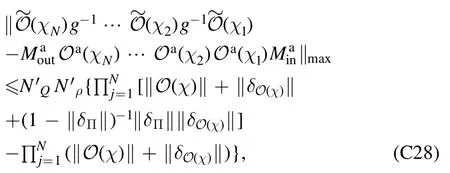
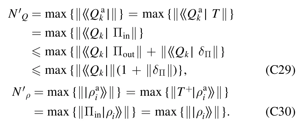
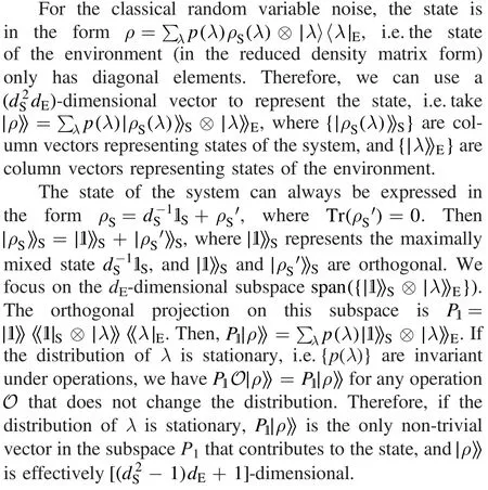
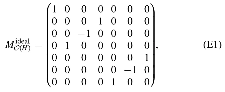
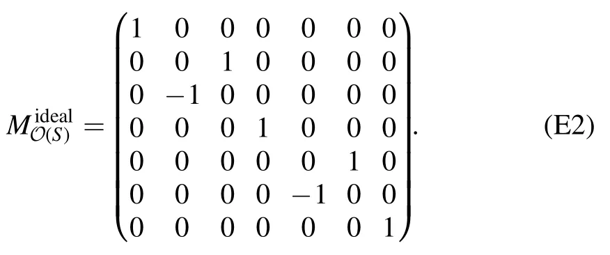
We consider the case that d

If‖∣ρi》‖≤Nρ,‖《Qk∣‖≤NQ,‖O(χ)‖≤NO,and‖ΠinO(χ)Πin-O(χ)Πin‖≤∊4We use‖·‖to denote a vector norm satisfying∣《A∣ B》∣≤‖《A∣‖‖∣B》 ‖and the submultiplicative matrix norm induced by the vector norm.We can take ‖∣·》‖=‖·‖1,where‖·‖1 is the trace norm.Then,‖O‖=1 ifO is tracepreserving.‖·‖max denotes max norm.,we have for an arbitrary sequence of elementary operations.See appendix B for the proof.Here,we always haveNO=1 by taking the trace norm.A small∊means that the subspace is approximately invariant under elementary operations,in which case an approximate tomography is possible.

There are various ways to find out the truncated dimension d

5.Approximate models of temporally correlated errors

The practical use of LOT requires that a low-dimensional approximate model exists.In this section,we consider two typical sources of temporal correlations,i.e.low-frequency noise and context-dependent noise.For both of them,lowdimensional approximate models exist.

5.1.Low-frequency noise and classical random variables

A typical source of temporally correlated errors in laboratory systems is the stochastic variation of classical parameters as discussed in section 2.For instances,in the trapped ion system,drifts of laser parameters cause time dependent coherent error[47];in the superconducting qubit system,fluctuations in the quasiparticle population lead to temporal variations in the qubit decay rate[57].If the correlation time of the noise is negligible compared with the time of a quantum gate,temporal correlations in gate errors are insignificant.However,if the correlation time is comparable or even longer than the gate time,errors are correlated,i.e.a sequence of quantum gates cannot be factorized because of low-frequency noise.We show that errors with this kind of correlations can be efficiently approximated using a low-dimensional model if moments of the parameter distribution converge rapidly.We remark that LOT is not limited to classical correlations and can be applied to general cases as long as the dimension truncation is valid.

As the same as in section 2,We can use

to describe a state that depends on random variables λ.Here,λ is an array with n elements that respectively denote n variables,and ρS(λ)is the state of the system when variables are λ.An operation depending on random variables reads

whereOS(χ,λ)is the operation on the system when variables are λ.Compared with the expression in section 2,there is an additional operation T(χ)in O(χ),which describes the stochastic evolution of variables in the time of the operation.HereT(χ)=[1S]⊗TE(χ),TE(χ)=∫dλ′dλtλ′,λ(χ)[∣λ′〉〈λ∣E],tλ′,λ(χ)is the transition probability density from λ toλ′,and 1 is the identity operator.Similarly,an observable depending on random variables reads

where QS(λ)is the observable of the system when variables are λ.

The approximate model is given by

Here,L is a finite subset of random variables.If λ takes m values in L,i.e.∣L∣=m,the environment in the approximate model is m-dimensional.The transition operation in the approximate model iswhereWe remark that ρS(λ),OS(χ,λ)and QS(λ)are the same as in equations(5)-(7).By properly choosing the subset of random variables L,the distribution pa(λ)and transition matricessuch a model can approximately characterize the quantum computer as we will show next.

We focus on the case of only one random variable,and the generalization to the case of multiple variables is straightforward.In a quantum computation platform,the effect of the noise on quantum operations should be weak,i.e.error rates are low.In this case,only low-order moments are important.Using the Taylor expansion,we have

Then,the quantum computation of a mean value,i.e.the mean of an observable Q in the state ρ after a sequence of operations,can be expressed as

where l=(l0,l1,…,lN,lN+1),λjis the value of the variable at the time of the jthoperation,and the overline denotes the average.Therefore,the behavior of the quantum computer is determined by correlations of random variables.If these correlations can be approximately reconstructed in the approximate model,the model approximately characterizes the quantum computer.

Correlations are formally defined here.We introduce the operatorThen,

whereρE=∫dλ p(λ)∣λ〉〈λ∣E.

5.1.1.Second-order approximation.First,we consider the case that the contribution of high-order correlations other thanλjandλ j′λjis negligible,the distribution of λ is stationary,and the correlation time is much longer than the time scale of a quantum circuit.In this case,onlyλjandλ j′λjare important.Without loss of generality,we assume that the distribution is centered at λ=0,i.e.λj=0.Because of the long correlation time,the change of the random variable is slow,andis approximately a constant.Such correlations can be reconstructed in the approximate model with m=2.We can take parameters in the approximate model as L={λ=±σ},pa(±σ)=1/2 and

Next,we consider the case that the correlation is not a constant but decreases with time.We assume that for each operation χ the correlation is reduced by a factor of eΓ(χ).If the correlation decreases exponentially with time,Γ(χ)is proportional to the operation time.The correlation readsThis two-time correlation can also be reconstructed in the approximate model with m=2.The only difference is the transition matrix.We take the transition matrix asand

5.1.2.High-order approximations and multiple variables.We consider the case that the change of the random variable is negligible in the time scale of a quantum circuit,i.e.TE(χ)≃[1E].Then,correlations becomeIf the contribution of correlations with l>ltis negligible,we only need to reconstruct correlations with l≤ltin the approximate model,which is always possible by taking m=(lt+1)/2[58].We remark that m is the dimension of the environment in the approximate model.

It is similar for multiple random variables.If moments of the distribution converge rapidly,the Gaussian cubature approximation can be applied[59].Then,up to-order moments can be reconstructed withwhere nλis the number of random variables.

5.2.Classical context-dependent noise

Context dependence is the effect that the error in an operation depends on previous operations,i.e.the environment has the memory of previous operations.Here,we consider the case that the environment has a record of the classical information about previous operations.Because this kind of effects is in the scope of our general model of the quantum computer in section 2,our results can be applied to the context-dependent noise.A list of previous operations is the classical information,so the memory of previous operations can be treated as a set of classical variables whose evolution is operationdependent.Therefore,we can use the same formalism for classical random variables to characterize the contextdependent noise.We consider two examples as follows.

In the ion trap,the temperature of ions may depend on how many gates have been performed after the last cooling operation,and the fidelity of a gate depends on the temperature.This effect can be characterized using a set of discretized variables λ=(n1,n2,…).Here,nidenotes the phonon number of the ithmode.Because of the low temperature of ions,each nican be truncated at a small number.Suppose the evolution of the qubit state mainly depends on the distribution at the beginning of the gate,the gate can be expressed as the same as in equation(9),where T(χ)describes the heating process in the gate χ.The cooling operation can also be expressed in this form.Then,we can apply the approximation similar to classical random variables.

If the error in an operation only significantly depends on a few previous operations,we can use a low-dimensional environment to characterize the effect.We focus on the case that the error only depends on the last one operation,and it can be generalized to the case of depending on multiple previous operations.We characterize this effect using one discretised variable λ∈{χ},where{χ}is the list of all possible operations.The state after the operation λ can be expressed in the formρ =ρS⊗∣λ〉〈λ∣E.An operation can be expressed in the formO(χ)=∑λOS(χ ,λ)⊗[∣χ〉〈λ∣E],whereOS(χ ,λ)is the operation on the system when the last operation is λ.After the operation,the state becomes O(χ )ρ=[OS(χ ,λ )ρS]⊗∣χ〉〈χ∣E.We remark that it is not necessary that∣λ∣Ecorresponds to a pure state in a physical Hilbert space.

6.Approximate quantum tomography

The exact tomography protocol is not practical because of the high-dimensional state space of the environment.In section 5,we show that an effective model with a low-dimensional environment state space can approximately characterize the quantum computer for typical temporally correlated noises.In this section,we discuss how to implement LOT to obtain a low-dimensional approximate model of the quantum computer.There are two approaches of self-consistent tomography,the linear inversion method(LIM)and the maximum likelihood estimation(MLE)[6,38–42],and we will discuss both of them.

6.1.Linear inversion method

Given sufficient data from the experiment,we can use LIM to obtain an exact model of the quantum computer as discussed in section 3.However,to obtain an approximate model,even if the approximate model exists,LIM does not always work.We suppose that d×d matrices,and{Oa(χ)}satisfy

for any sequence of elementary operations.See appendix C for the proof.Therefore,LIM works under conditions thatand∊gand∊Oare small quantities.

We apply this result to the approximate model given by the approximately invariant subspace Πin.We have for any sequence of elementary operations.See appendix C for the proof.Here,∊Π=‖Πin-Πout‖,and we haveNO=1 by taking the trace norm.Therefore,if‖ΠinO(χ)Πin-O(χ)Πin‖≪1and‖Πin-Πout‖≪1for the trace norm,LIM can be applied.Here,‖Πin-Πout‖≪1 means that two subspaces Πinand Πoutare approximately the same.

The approximate LOT protocol using LIM is as follows:

6.2.Maximum likelihood estimation

We can parameterize the error model by taking each vector and matrix element as a parameter.If the main source of temporal correlations is low-frequency noise or contextdependent noise as discussed in section 5,we can parameterize the error model according to equations(8)-(10).Choosing the proper initial values of parameters is important in the MLE method,and it is convenient to implement LIM and take the result of LIM as the initial values.

7.Numerical simulation of low-frequency noise

We consider two single-qubit gates,the Hadamard gate H and the phase gate S,which can generate all single-qubit Clifford gates.We take∊H(λ)=∊S(λ)=η[1 -exp(-λ2)],therefore,two gates are both optimised at λ=0.Here,η∈[0,1]denotes the strength of the noise.RB is the usual way of the verification of a quantum computing system[7,8,10].In our simulation,we perform a sequence of H and S gates randomly chosen in the uniform distribution.We initialize the qubit in the state∣0∣,perform the random gate sequence and measure the probability in the state∣0∣.We only take into account gate sequences that the final state is∣0∣in the case of ideal gates without error,so that the probability in the state∣0∣is expected to be 1.When errors are switched on,the probability in the state∣0∣isif η=1,where Ngis the number of gates in the random gate sequence.The non-exponential decay of the probability is due to temporal correlations[7–13].Without temporal correlation,the probability decreases exponentially with the gate number.If depolarizing rates are constants,i.e.∊H(λ)=∊S(λ)=∊,we have [1+(1-∊)Ng]2.

In our simulation,we implement both LIM and MLE.We take the dimension of the state space d=4,7 to compare LOT with conventional GST.In approximate models of classical random variables with stationary distribution(see section 5.1),the state space is-1)m+1]-dimensional when the system and environment Hilbert spaces are respectively dS-dimensional and m-dimensional,as explained in appendix D.Therefore,d=4,7 correspond to m=1,2 approximations,respectively.If d=4,the LOT protocol is equivalent to conventional GST protocol,because the onedimensional environment is trivial and does not have any effect.As shown in figure 2,LOT with d=7 can characterize the behavior of the quantum computer much more accurately than LOT with d=4(i.e.conventional GST).We remark that the Hilbert space dimension of the environment is infinite in the error model used in the numerical simulation,and the full tomography of the entire Hilbert space using informationallycomplete states and observables is impractical.The number of measurements needed in the tomography increases with the dimension of space.In our method,when we truncate the space dimension to d=7,we can already reconstruct an approximate error model that is consistent with the behavior of the quantum computer with temporal correlations.

In the simulation of LOT using MLE,we parametrize the state,observable and operations as follows.The state is in theformThe observable is in the formThe gate G with error is in the formWe take{pa(λ)}andas parameters(i.e.x)in MLE.With the error model parametrized in this way,the number of values that λ can take is important,but the value of λ is not important.For the one-dimensional environment approximation,i.e.d=4,we take L={1};and for the two-dimensional environment approximation,i.e.d=7,we take L={1,2}.Using MLE,we obtain pa(1)=0.5606,pa(2)=0.4394,=2.485×10-3and1.606×10-2.

Figure 2.Probabilities in the state∣0∣after a sequence of randomly chosen Hadamard and phase gates as functions of the gate number.We initialize the qubit in the state∣0∣,perform the random gate sequence and measure the probability in the state∣0∣.We only take into account gate sequences that the final state is∣0∣in the case of ideal gates without error.Therefore the probability should be 1 in this case.In our simulation,we take σ=1 and η=0.02.In the presence of errors,the probability in the actual quantum computation(QC)decreases with the gate number(black curve).Based on error models obtained in linear operator tomography(LOT)using MLE,we can estimate the decreasing probability,and the results are plotted.We can find the that the error model with d=7(red crosses)fits the actual behavior of the quantum computer much more accurately than the error model with d=4(blue squares).When d=4,LOT is equivalent to conventional GST.Results for the linear inversion method are similar.See appendix E for details of the simulation and more data.

In the case that the random variable takes two values λ=1,2,the environment state isBecause the distribution is stationary,the state of the environment does not evolve.Usually,we can use an eight-dimensional Pauli transfer matrix to represent an operation on a qubit and a classical bit[6].However,because the componentis always zero(see appendix D),the dimension of the state space is effectively seven.For the operationO,the corresponding seven-dimensional Pauli transfer matrix isMO;σ,τ=Tr[σO(τ)]2,wherePauli transfer matrices obtained using LIM are show in figure 3.In figure 4,we show the error in probabilities in the ideal state|0>estimated using different methods.

8.Conclusions

We have proposed self-consistent tomography protocols to obtain the model of temporally correlated errors in a quantum computer.Given sufficient data from the experiment,the model obtained in our protocol can be exact.We also propose approximate models for the practical implementation.To obtain approximate models characterizing temporal correlations,more quantities need to be measured compared with conventional QPT and GST,but the overhead is moderate.We can use such approximate models to predict the behavior of a quantum computer much more accurately than the model obtained in GST,for systems with temporally correlated errors.Our protocols provide a way to quantitatively assess temporal correlations in quantum computers.

Acknowledgments

This work was supported by the National Key R&D Program of China(Grant No.2016YFA0301200)and the National Basic Research Program of China(Grant No.2014CB921403).It is also supported by Science Challenge Project(Grant No.TZ2017003)and the National Natural Science Foundation of China(Grants No.11 774 024,No.11 534 002,and No.U1530401).YL is supported by National Natural Science Foundation of China(Grant No.11 875 050,12088101)and NSAF(Grant No.U1930403).

Appendix A.Exact LOT

Lemma 1.Let O∈O,all the following expressions are valid.

Proof.We have

Therefore,equation(A1),equation(A2)and equation(A3)are valid.

UsingOPin=PinOPinandPoutO=PoutOPout,we have

Similarly,

Therefore,equation(A4)is valid.

Theorem 1.Let∣σ》∈Vin,《H∣∈VoutandOi∈O,where i=1,2,…,N.Then,

Proof.Using lemma 1,we have

and

Figure 4.The difference between probabilities in the ideal state∣0∣after a sequence of randomly chosen gates.(a,b)The probability difference Ftom-Fact,where Fact is the probability obtained in the actual quantum computing,and Ftom is the probability estimated using linear operator tomography(LOT).The errorbar denotes one standard deviation.

Using∣σ》=Pin∣σ》and《H∣=《H∣Pout,we have

Similarly,

We also have

Therefore,the first two lines of equation(A16)are equal.

Using pseudo inverses,we haveg-1=(PMin)+(MoutP)+,i.e.g=is invertible.Thus,

Therefore,the last two lines of equation(A16)are equal.

Appendix B.Space dimension truncation

We use‖·‖maxto denote the max norm.

Lemma 2.LetNQ≥‖《Qk∣‖for all k,andNρ≥‖∣ρi》 ‖for all i.Then

According to the property of vector norm,the proof of lemma 2 is straightforward.

Theorem 3.LetNQ≥‖《Qk∣‖for all k,andNρ≥‖∣ρi》 ‖for all i.Then,for any sequence of operations,

where

Proof.Inequality(B2)holds for n=0,because

If inequality(B2)holds for n=m,then it also holds for n =m +1.Now we assume that inequality(B2)holds for n=m.Because

we have

Because

we have

i.e.inequality(B2)holds forn =m +1.

Appendix C.Linear inversion method

where

Proof.We have

Then,

Therefore,inequality(C1)holds.

Because

we have

LetO be an operation satisfyingΠinOΠin=T+OaT,we have

where

We have,

Therefore,δg=0.

We have

Then,

Then,

We define δΠ≡Πin-Πout.If 1-δΠis invertible,we have

Then,

Therefore,

Using inequality(C1),we have

where

Appendix D.Vector space dimensions

If Hilbert spaces of the system and environment are respectively dS-dimensional and dE-dimensional,the Hilbert space of SE is(dSdE)-dimensional.Then,a column vector∣ρ》representing the state of SE is()-dimensional.We remark that dE=m.

Appendix E.Details of the numerical simulation

E.1.Actual quantum computer simulation

To simulate the behavior of the actual quantum computer,we use the Gaussian cubature approximation to match up to the 9th-order moment,by taking-λe2instead of λ as the random variable.Reducing the precision of the approximation and only matching up to the 7th-order moment,we find that the difference is negligible.

E.2.Linear inversion method simulation

Trial states and observables are generated as follows:We selected a set of gate sequences,(G1,G2,…,GN),where Gj=H,S;Each gate sequence corresponds to a stateGN…G2G1∣0∣and an observable(G1G2…G N)†Z(G1G2…GN).These states and observables are realised using H and S gates accordingly.

When d=4,four gates sequences are used in the simulation,(null),(H),(H,S)and(H,S,H).The four states are∣0∣,∣+∣=H∣0∣,∣y+∣=SH∣0 ∣and∣y-∣=HSH∣ 0∣;The four observables are Z,X=H†ZH,-Y=S†H†YHS and Y=H†S†H†YHSH.

When d=7,123 gates sequences are used in the simulation,including all sequences with the gate number N≤5 and four sequences for each gate number 5

E.3.MLE simulation

Circuits for generating data{Cm}used in MLE are the same as circuits used in LIM simulation.

E.4.Pauli transfer matrices

The seven-dimensional Pauli transfer matrices of ideal gates are

and