Impacts of household income on beef at-home consumption:Evidence from urban China

ZHU Wen-bo,CHEN Yong-fu,ZHAO Jing,WU Bei-bei

1 College of Economics and Management,China Agricultural University,Beijing 100083,P.R.China

2 Appalachian Laboratory,University of Maryland Center for Environmental Science,Maryland 21532,USA

3 College of Economics and Management,Nanjing Agricultural University,Nanjing 210095,P.R.China

Abstract Beef consumption in China has increased substantially from 5.0 million tons in 2000 to 7.7 million tons in 2019 thanks to rapid income growth,but still remains low compared to pork and poultry consumption. Improving the understanding about the impacts of household income on beef consumption in China is necessary to forecast future beef demand and inform the domestic beef industry,especially in the context of unprecedented expansion of middle income class in China.Based on survey data of 32 878 urban households collected by the National Bureau of Statistics of China,we employed the inverse hyperbolic sine (IHS) double-hurdle model to estimate income elasticities of beef demand across different income groups and simulated possible trends of future beef consumption of Chinese urban residents. The empirical results showed that the unconditional income elasticities of beef consumption at home vary between 0.169 for the lowincome group and 0.671 for the high-income group. The simulated results indicated that beef consumption is expected to increase by 12.0 to 38.8% in 10 years and by 18.6 to 70.5% in 15 years under distinct income growth scenarios. Our findings provide practical insights for policy makers and other stakeholders about future beef demand,such as potential opportunities embedded in rising beef demand for domestic producers and world beef exporters as well as the urgency of improving the supply chain resilience of beef in China.

Keywords:beef consumption,income elasticity,income growth,IHS double-hurdle model,urban China

1.Introduction

In China,the traditional fiber-dominated food system is being replaced by a Western-style meat-dominated diet mainly because of the rapid economic growth and drastic nutrition transition (Popkin 2006;Huang and Gale 2009;Yu and Abler 2009;Gandhi and Zhou 2014;Yu 2015;Huanget al.2017;Zhenget al.2019). According to the OECD-FAO (2019),China’s beef consumption reached 7.7 million tons in 2019,a 55% increase from 2000,which accounted for 11% of global consumption. However,per capita beef consumption in China is less than 16% of the consumption level in the United States and Australia (FAO 2020). With its large population,a small change in per capita consumption in China could have a tremendous impact on total national beef consumption. Therefore,beef consumption is expected to have the largest growth potential among different meats in China because of consumers’ changing purchasing power,attitudes and taste preferences toward beef (Maoet al.2016;Zhenget al.2019). Meanwhile,China’s beef import dependence is rising because it has limited capacity to increase domestic beef production due to the land,feed,water,and environmental constraints (Sunet al.2015;Baiet al.2018). China’s beef net imports had been soaring by 3-fold in past five years from 0.3 million tons in 2014 to 1.3 million tons in 2019,which made China the fastestgrowing beef importer in the world (OECD-FAO 2019).Therefore,investigating the potential of future beef demand in China is critical for multiple stakeholders in China and all over the world.

Moreover,urban households’ strong demand for highquality meat products is the most important driver of beef consumption in China (Zhenget al.2016). In 2019,beef consumed by urban residents (60.6% of total population)accounted for more than 79.1% of China’s total beef consumption. Per capita beef consumption in urban areas was 2.7 kg in 2018,while that in rural areas was only 1.1 kg (NBSC 2019). Additionally,urban population expanded from 669.8 million in 2010 to 848.4 million in 2019 and is projected to reach 1.09 billion by 2050(UNDESAPD 2018). Therefore,this paper mainly focuses on urban households and offers new evidence for the growing trends of beef at-home consumption of Chinese urban residents.

Previous studies have comprehensively examined the determinants of beef consumption,such as income,price,household composition,and some demographic characteristics (Gould 2002;Maet al.2004;Minet al.2015). Income is the key determinant of beef consumption in China and the world (Chern and Wang 1994;Gale and Huang 2007;Sealeet al.2012;Bilgic and Yen 2013). Many studies have proven that increased income can increase consumers’ beef consumption (Gould and Dong 2004;Hovhannisya and Gould 2011). In our sample,the average annual beef consumption at home of the medium-and high-income urban households are 1.45 times and 1.61 times that of the low-income group,respectively,reflecting the important role of income in beef consumption (Zheng and Henneberry 2010,2011).Furthermore,different income groups have distinct preference patterns (Leibenstein 1975). Compared with consumers in the low-income group,those in the highincome group prefer more high-quality food and have a stronger capability to increase their diet diversity,such as including beef that has more high-quality protein and less fat than pork (Chenet al.2014;Zhanget al.2018).

According to the theory of consumer behavior in economics,demand elasticity analysis indicates how beef consumption responds to changes in income,and the estimated income elasticity can be used to simulate the trends of beef consumption (Deaton and Muellbauer 1980). In a meta-analysis of 85 studies on food consumption,Chenet al.(2016) found that the unconditional income elasticity of China’s beef consumption ranges from–0.253 to 1.583,with a mean value of 0.636. The variations in estimated income elasticities could be attributed to different models,data,and estimation methods. For instance,previous published studies usually used aggregated data or focused on a certain region,such as a province or several cities,lacking of the in-depth research of beef consumption based on more widely distributed data with a large sample size in urban China (Yenet al.2004;Gale and Huang 2007;Sealeet al.2012;Ulubasogluet al.2016;Zhenget al.2016;Zhenget al.2019). Additionally,the heterogeneity of beef consumption across income groups further amplifies the uncertainty of income elasticity estimation (Zheng and Henneberry 2011). Furthermore,except elasticity estimation,there is a general paucity of studies that have conducted a simulation for capturing the possible trends of beef consumption with more accurate information on income elasticities across detailed income strata.

However,the zero consumption problem often exists in widely distributed micro data with large sample sizes,which may cause biased estimates in food demand (Yen and Huang 1996;Shonkwiler and Yen 1999). The Tobit model,the standard double-hurdle model,and Heckman’s two-step procedure are commonly used to address the problem of zero consumption and obtain unbiased parameter estimates (Fulleret al.2007;Baiet al.2008;Zheng and Henneberry 2010,2011;Wuet al.2014).However,they all have limitations and perform poorly when the normality assumptions are violated,resulting in inconsistency in the maximum likelihood estimator (Yen and Huang 1996). Fortunately,a generalized doublehurdle model with the inverse hyperbolic sine (IHS)transformation can accommodate both nonnormality and the problem of zero consumption simultaneously(Jensen and Yen 1996;Yen and Huang 1996;Jones and Yen 2000;Rudeet al.2014;Chenet al.2018). This model can measure the consumption decision process of beef more accurately than the aforementioned model because it has been shown to adequately characterize the two processes in consumption:participation and then consumption (Zhanget al.2008). Since micro data used in this study contains 32 878 urban households of which 13% have zero expenditure on beef consumed at home,an IHS double-hurdle model was used in this study.

The goal of this paper is to estimate the income elasticities of beef demand across different income groups in urban China by using IHS double-hurdle model and then simulate the possible trends of beef consumption in distinct income growth scenarios. We have two main academic contributions to the literature. First,this study is among the first to apply a generalized double-hurdle model with IHS transformation to estimate China’s beef consumption at home considering both participation process and consumption process. Second,this paper applies distinct income elasticities across one hundred income groups in the simulation and demonstrates the differences of estimated beef consumption with that obtained when only one income elasticity is considered for the whole population.

The structure of this paper is as follows. Section 2 presents the methodology and data. In Section 3,the empirical results and simulation results are presented.Section 4 is the discussion while Section 5 is the conclusion.

2.Methodology and data

2.1.IHS double-hurdle model

Following the method of Yen and Huang (1996) and Yen and Jones (1997),the decision of beef consumption can be divided into two stages. Urban residents decide their probability to participate in the beef market in the first stage,and then decide the quantity of beef consumption in the second stage (Wooldridge 2002;Wuet al.2014;Chenet al.2018). The specifications of the model are as follows:

Equations (1) and (2) represent the participation equation and consumption equation of householdi,respectively,in whichare latent participation indicator and latent consumption of beef consumption,respectively;y2iis observed beef consumption and ifand,then;otherwise,y2i=0.are vectors of explanatory variables,which are determinants of beef consumption,in the participation equation and consumption equation,respectively;β1andβ2are vectors of parameters to be estimated;andμ1iandμ2iare error terms.

Additionally,we assume thatμ1iandμ2iare distributed as the binary normal distribution and that their covariance isρσ,andμ1iis normalized to unity:

In general,the double-hurdle model can be estimated by using maximum likelihood estimation (MLE) assuming a binary normal distribution of error terms. However,if this assumption is invalid,MLE generates inconsistencies.Therefore,the conditional moment (CM) test developed by Skeels and Vella (1999) is used to test whether the normality assumption is violated. Additionally,IHS transformation can also be used to address the issue of violating normality as well as the problem of zero consumption simultaneously (Jensen and Yen 1996).Specifically,the dependent variable of the model (yi) is converted toyi Tby using IHS transformation:

whereθis an unknown parameter to be estimated. If the null hypothesisθ=0 is rejected,the assumption of a normal distribution is violated and the IHS transformation is appropriate. According to eqs.(1),(2),and (4),the relationship betweenyi Tand the latent variables of beef consumption can be summarized as:

Based onnindependent observations and parameters to be estimated (β1,β2,ρ,σ),the likelihood function of the IHS double-hurdle model can be expressed as:

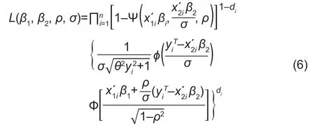
where Ψ(·) is the cumulative density function of the binary standard normal distribution and the covariance isρσ;φ(·) and Φ(·) are the probability and cumulative density function of the normal distribution,respectively.diis the dichotomous index,withdi=1 ifyi＞0anddi=0 otherwise(Gaoet al.1995).

To correct the potential heteroskedastic errors that usually cause inconsistency of parameter estimates in limited dependent variable models,this study assumes that heteroscedasticity is present in the variance (σ) of the error term of eq.(2) (Greene 2004). The specification of the heteroscedasticity equation is as follows:

wiis the vector of the subset of the explanatory variablesx2i,andλis the vector of corresponding parameters.Thewiof the heteroscedasticity equation is determined through the test of the null hypothesis ofλ=0 (Brownet al.2015).

In the double-hurdle model,the total or unconditional effectE(yi) can be decomposed into the effects on the probability of participationP(yi＞0) and the conditional level of consumptionE(yi|yi＞0),which leads to considerably complicated calculations of marginal effect and elasticity(McDonald and Moffitt 1980;Yen and Huang 1996).Using the IHS transformation to estimate the parameters of eqs.(1),(2),and (7) through MLE has also increased the complexity. The details of the partial derivative process are in Chenet al.(2018).

After calculating the partial derivatives ofP(yi＞0),E(yi|yi＞0),andE(yi) with respect to each continuous variable,the average elasticity of variablejcan be calculated by using eqs.(8),(9),and (10).

The marginal effect of a binary variable is the difference ofP(yi＞0),E(yi|yi＞0),andE(yi) when the binary variable changes from 0 to 1 (McDonald and Moffitt 1980;Jones and Yen 2000),using eqs.(11),(12),and (13):

2.2.Simulation method

To demonstrate the possible trends of beef consumption in urban China and show the necessity and importance of considering income elasticities by income groups on the simulation results,this study conducted a simulation based on the accurate information of income elasticities and the growth rates of income across different income groups. We also considered a dynamic process through which households enter a higher income group as their income increases,so that the simulation is close to reality.

Compared with the baseline level,the growth rate of beef consumption (ΔQT) in the followingtyears (t=1,…,15) resulting from different income elasticities and income growth rates can be expressed as follows:

It should be noted that four assumptions must be made to perform the simulations. First,the households in each income group are assumed to have constant preferences.Second,the prices are assumed to remain unchanged over time. Third,the effects of other determinants such as household composition on beef consumption are not considered because these impacts are very small compared with those of increased income. Fourth,the total number of households is assumed to remain unchanged (Zheng and Henneberry 2010).

2.3.Data and selected variables

Our data are mainly from the 2007–2009 urban household survey conducted by the NBSC,except for the latitudes from city administrative offices. The NBSC household survey data,which contain both permanent urban households and rural migrants and have been widely used in empirical studies of China’s urban food demand,represent all income classes in urban China(Yenet al.2004;Gould and Villarreal 2006;Zheng and Henneberry 2011;Han and Chen 2016;Chenet al.2018).Our sample data reflect the regional differences through 32 878 urban households from 224 cities of Hebei Province (sample size,4 919;region,north),Jilin Province(2 925,northeast),Henan Province (6 934,central),Guangdong Province (7 536,south),Sichuan Province(7 481,southwest),and Xinjiang Uygur Autonomous Region(3 083,west). The NBSC survey data capture consumption and expenditures through a diary kept by the chosen households over a one year period and can thus reflect accurate beef consumption characteristics (Gould 2002;Zheng and Henneberry 2011;Hanet al.2019).Therefore,the key variables used in this study,such as the beef consuming quantity and household income,are all representing the sum value of a whole year for a household.

A major goal of this study is to estimate the income elasticities of beef demand across different income groups. To accomplish this goal,we categorized our samples into low-,medium-,and high-income groups based on household income,following NBSC’s classification standards for urban households (Zheng and Henneberry 2010). Specifically,ranking all households in the descending order of income,the low-income group refers to households in the lowest 20% income bracket,the high-income group refers to those in the highest 20%and the medium-income group refers to the remaining portion of the samples (Wanget al.2014). The ranges of household income in the low-,medium-,and high-income group are 21.2–3 408.0 USD,3 408.1–9 122.5 USD,and 9 122.8–97 140.5 USD,respectively. The summary statistics for the major variables by income group are presented in Table 1.

In the full sample,13% of households have zero beef consumption. Additionally,the proportions of households with zero beef consumption from the low-,medium-,and high-income group are 17.18,12.80,and 9.02%,respectively,which are higher than those reported by Gould and Villarreal (2006) (0.4%) but lower than those of Yenet al.(2004) (18.9%),Liu and Chern (2004) (20.7%),and Liuet al.(2009) (30%). The dependent variable is annual household beef consumption,which is 7.316 kg on average for the whole sample,and 8.401 kg if excluding households with zero consumption (Table 1).The average consumption in the low-,medium-,and highincome group is 5.245,7.630,and 8.433 kg,respectively,and 6.333,8.751,and 9.268 kg,respectively,if excluding households with zero consumption.

A number of earlier studies have demonstrated that income is the most important economic driver of beef consumption (Chern and Wang 1994;Maet al.2004;Chenet al.2016). Additionally,existing studies have conducted detailed analyses of different income classes(Gould and Villarreal 2006;Huang and Gale 2009;Zheng and Henneberry 2011;Sealeet al.2012). The annual total household incomes of the low-,medium-,and highincome groups are 2 828,6 093,and 12 404 USD (Fig.1),and the coefficients of variation are 0.464,0.392,and 0.486,respectively. Household income is not normally distributed since the mean value is larger than the median income for the full sample and different income groups(Fig.1). Therefore,to minimize the bias caused by applying one income elasticity for the whole population(Zheng and Henneberry 2011),we simulated beef consumption with separate income elasticities for differentincome groups.

Table 1 Summary statistics for major variables1)

Price is another key factor of beef consumption. The effects of own-price and cross-price on food demand in the literature have been examined (Gould and Dong 2004;Zheng and Henneberry 2010;Chengappaet al.2016).For the price variables,similar to Cox and Wohlgenant(1986) and Gaoet al.(1995),a quality-adjusted price was used. First,this study calculated the unit value of beef by dividing beef expenditure by the quantity of beef consumed. Second,based on the unit value without including the quality factors,the quality-adjusted price was calculated by using the hedonic price regression (Cox and Wohlgenant 1986;Gaoet al.1995). The qualityadjusted beef price ranges from 2.554 to 2.585 USD kg–1for the total sample and three income groups. Similarly,the quality-adjusted prices of other meats including pork,mutton,and poultry were calculated and presented in Table 1.

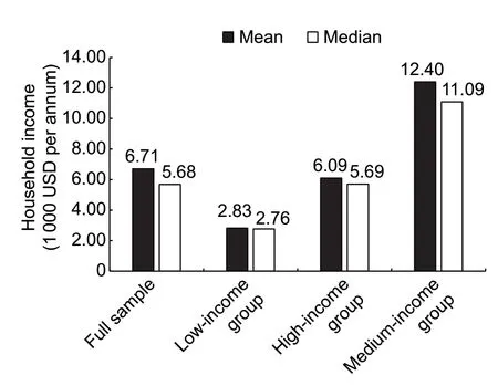
Fig.1 Mean and median of household income for the full sample and different income groups. Source:Calculated based on the NBSC (National Bureau of Statistics of China) household survey data used in this study.

As for the control variables,we included household composition,ethnic,city latitudes,provincial beef production,dining out expenditure,home ownership,refrigerator ownership,and year dummy variables (Gould 2002;Zhonget al.2012;Minet al.2015;Chenet al.2018). As shown in Table 1,urban households were divided into eight categories based on gender and age to show the features of household composition. The ethnic variable indicates whether a household head belongs to the Han ethnic group. Households headed by Han people account for 94.9% of the full sample. Latitudes of the sample cities were used to reflect the south-north differences in beef consumption,which are caused by the geographical environment and dietary habits that have formed throughout its long history (Song and Cho 2017).In the full sample,the latitude has a range between 21.192 and 48.061 degrees,with a mean value of 33.108,which essentially spans most of northern and southern China.Furthermore,we included provincial beef production as an independent variable because natural endowment forms dietary habits of local people in many cases and the distribution of beef production across China may lead to differences in beef consumption. The average provincial beef production for the full sample is 0.41 million tons.Additionally,the proportion of food expenditures made away from home (FAFH) was added to the demand model for evaluating the potential impact of dining out on athome beef consumption per household (Baiet al.2020).Of total food expenditure,the average household share of dining out is 16.1% in our sample. Additionally,68.0% of urban households are homeowners,who own the property rights of the house. Owning a refrigerator makes storing beef at home convenient and the households having at least one refrigerator account for 90.0% of the sample.We included two year dummy variables,and observations in 2007,2008,and 2009 constitute 18.2,41.1,and 40.7%of the sample,respectively.

3.Results

3.1.Empirical results

Estimation resultsThe parameters of the IHS doublehurdle model in eqs.(1) and (2) were estimated through MLE in eq.(6),and the estimated results of Model 1 are shown in columns 2 to 5 of Table 2. Additionally,an IHS double-hurdle model accommodating heteroscedastic errors using eqs.(6) and (7) was estimated by MLE simultaneously. The variables included in eq.(7) are income and the ethnic variable,which are shown in columns 6 to 9 of Table 2 as Model 2. A Tobit model (Model 3)was also estimated by using MLE and the results are presented in columns 10 and 11 of Table 2. In addition,standard errors were calculated with 10 000 bootstrap replications and presented in Table 2 (Bilgic and Yen 2013;Pieroni and Salmasi 2014;Lucaset al.2018).

The test results of the model selection are presented in Table 2. All three parameters in eq.(7) in Model 2 are statistically significant at the 1% level,indicating that errors of the model are not homoscedastic and the double-hurdle model is preferred to accommodate heteroscedastic errors. The estimate of the IHS parameter (θ=0.267)is significantly different from zero at the 1% significant level. This finding shows that Model 2 is preferred compared with Models 1 and 3,which is consistent with the results of the following likelihood ratio (LR)tests. Furthermore,the CM test results shown in row 1 reject the null hypothesis that the error term is normally distributed significantly at the 1% level,which indicates that the application of IHS transformation is preferred.Therefore,the IHS double-hurdle model accommodating heteroscedastic errors (Model 2) is most preferred to estimate the impacts of selected variables on at-home beef consumption in urban China. Hence,the following analysis of empirical results is based on the estimated results of Model 2.

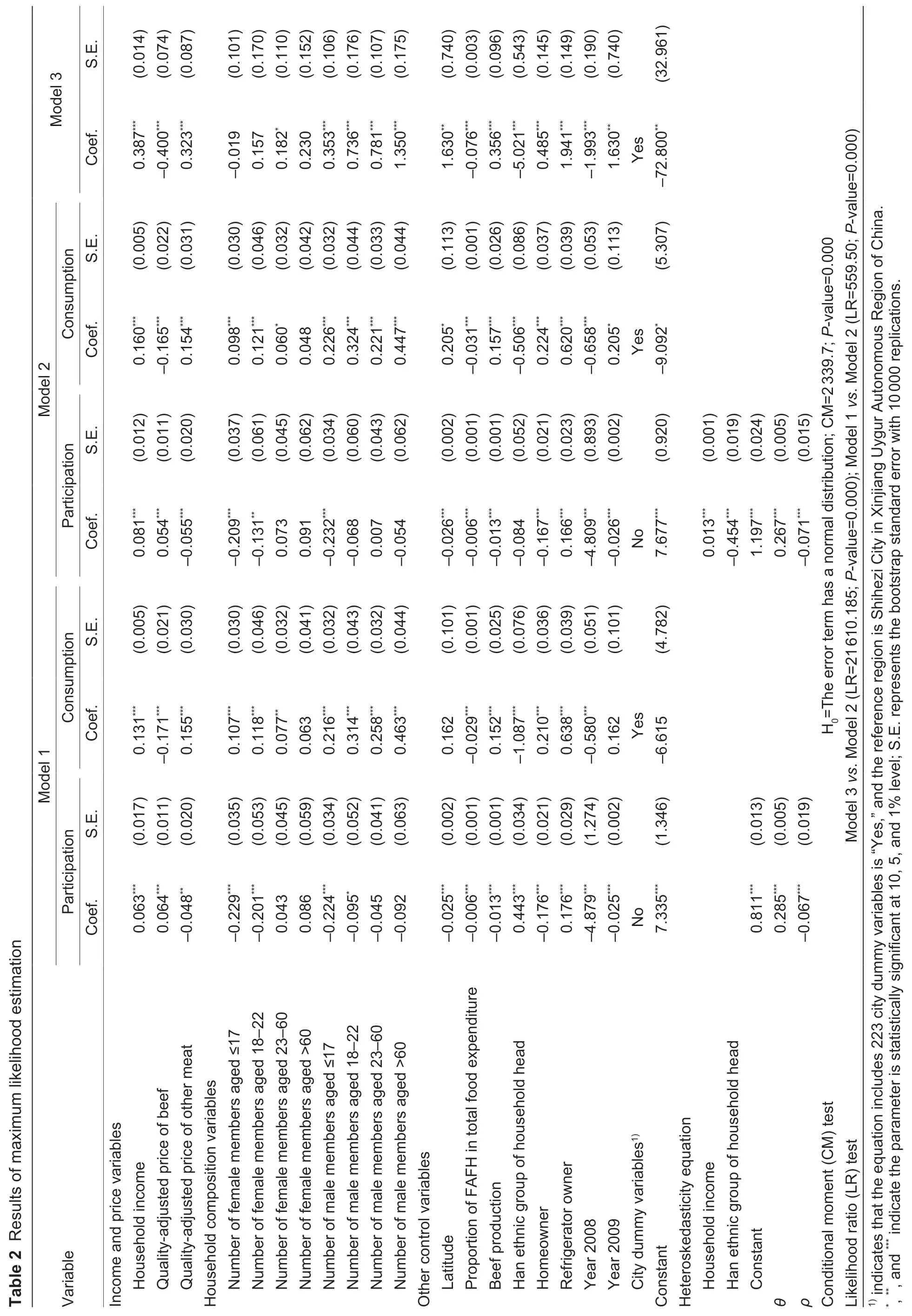
The main results are shown in Table 2. The estimation results in columns 6 to 9 of Model 2 show that income has a positive effect on beef consumption,at the 1% significance level,in both the participation and consumption equations,which is as expected and illustrates possible trends in beef purchasing probability and beef consumption when household income grows.As for price variables,household composition variables and other control variables,12 coefficients are statistically significant at the 1% level and 1 coefficient is at the 5%level in the participation equation. In the consumption equation,14 coefficients are statistically significant at the 1% level and 4 coefficients are at the 10% level. In addition,the correlation coefficient ofρ(=–0.071) between the participation equation and the consumption equation is statistically significant at the 1% level.

Elasticity and marginal effectThe average elasticities of the probability,conditional level,and unconditional level for continuous variables were estimated by eqs.(8),(9),and (10). As for binary variables,the corresponding marginal effects were estimated by eqs.(11),(12),and(13). Additionally,the estimated elasticities and marginal effects based on the full sample and three subsamples are presented in Table 3.

In Table 3,the income elasticities of the probability,conditional level,and unconditional level of beef consumption at home for the full sample are statistically significant at the 1% level. This finding indicates that a 1% increase in household income results in a 0.385%increase in beef consumption. The unconditional elasticities of beef consumption with respect to income in low-,medium-,and high-income households are 0.169,0.353,and 0.671,respectively,which indicates a rising trend as income increases. The elasticity estimation results are consistent with the MLE results and may be explained by the fact that consumers can expand their consumption market and liberate the consumption potential of high-quality beef with increased income.When consumers become less limited in their choice of various beef products available on the market,they are more sensitive to changes in income (Huang and Rozelle 1998). Furthermore,some studies have also concluded that the income elasticity of meat products for the high-income group is higher than that for the lowincome group (Fanet al.1994;Maet al.2004;Liuet al.2009;Chenet al.2018).

Compared with previous literature linking beef consumption with income,on the one hand,the unconditional income elasticities in this study are all in the range of–0.06 to 0.93 reported by Shonoet al.(2000),Gale and Huang (2007),Hovhannisya and Gould (2011),and Chen (2010) on China’s urban beef consumption;on the other hand,our unconditional income elasticity for the full sample (0.385) is more elastic compared to 0.05 reported by Okrent and Alston (2012) but less elastic relative to 0.458 by Parket al.(1996) on US beef consumption. Obviously,income elasticities provide strong evidence for the continuing growth of beef consumption in China during its transition from an uppermiddle income country to a high-income country (Song 2015).

The results also show that the income elasticities of beef vary significantly across income groups. Therefore,in order to simulate the changing trends of beef consumption more accurately,the sample data were divided into more income groups. Based on 32 878 observations and the method for dividing the low-,medium-and high-income groups presented before,the full sample households were divided into 100 income groups. The unconditional income elasticities were estimated by eqs.(8),(9),and (10) for each income group.

Fig.2 illustrates the income elasticities of beef consumption and the 99% confidence intervals. In Fig.2,the unconditional income elasticities have a range of 0.053 to 1.095 across the 100 income groups,showing an upward trend as income increases. This finding supports the previous elasticity results and provides strong evidence that beef consumption will continue to expand with income growth. Thus,we simulated the possible trend of China’s beef consumption considering different income elasticities across 100 income groups.

For the full sample,the own-price elasticity of athome beef consumption is inelastic with–0.134 at the unconditional level (Table 3). Meanwhile,the own-price elasticities across income strata show a rigid feature,which varies from–0.140 to–0.128. The cross-price elasticities for other meats at the probability,conditional level,and unconditional level are 0.011,0.098,and 0.109,respectively,which suggests that beef demand is not particularly responsive to other meats’ price changes(Gould and Dong 2004;Gould and Villarreal 2006).

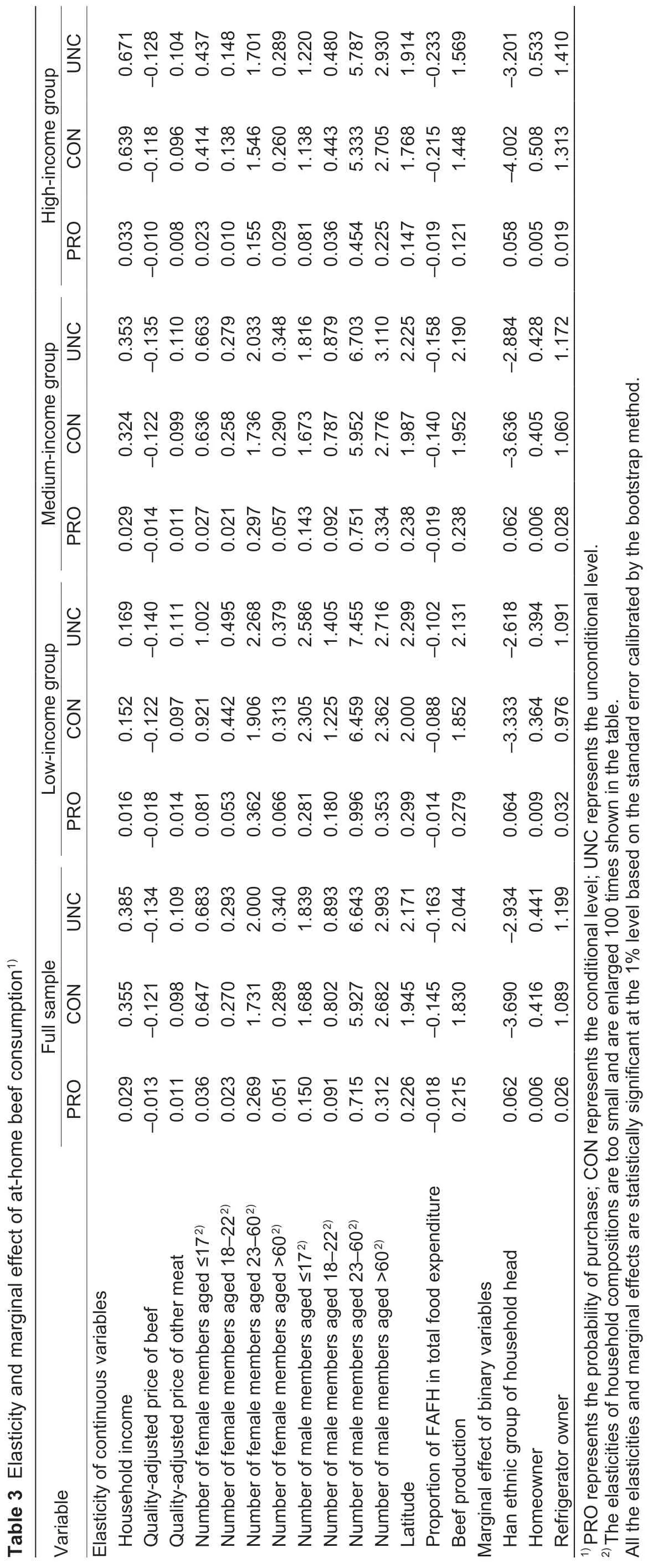
Household composition variables have positive effects on beef consumption of urban residents. First,the probability,and conditional and unconditional elasticities of household composition variables are positive. Second,the elasticities of household composition at the unconditional level take on an inverted U-shaped curve from the young age group to the old age group.Additionally,there is evidence that the older group consumes less beef than the middleaged group;thereby beef consumption could dwindle with societal aging,which is consistent with the findings of Minet al.(2015).

With respect to other variables,at-home beef consumption of urban households with a Han ethnic head at the conditional and unconditional levels is 3.690 and 2.934 kg lower than that of those with a minority head,respectively. The elasticities of at-home beef consumption with respect to latitude at the probability,conditional level,and unconditional level are 0.226,1.945,and 2.171,respectively. Additionally,the unconditional elasticities of beef demand with respect to dining out and beef production are–0.163 and 2.044,respectively,which indicate that a 1% increase in the share of dining-out and the provincial beef production would result in 0.163% decrease and 2.044% increase in beef consumption at home,respectively.Lastly,owing a home or a refrigerator has positive effects on beef consumption of urban residents,with the unconditional marginal effects being 0.375 and 1.178 kg,respectively.

RobustnessAlthough the model selection and a bootstrap standard error with 10 000 replications were processed,a robustness testing for control variables was further conducted through Robust model 1,Robust model 2,and Robust model 3,which are presented in Table 4. Robust model 1 only retained income,price variables,and city dummy variables. The household composition variables were added in Robust model 2,and the geographical,production and dining out variables were further included in Robust model 3. Table 4 shows that the estimated income elasticity and own-price elasticity of beef consumption at home in three robust models are both significant at the 1% level.In all three robust models,income elasticities have positive signs,and own-price elasticities are negative and vary within in a smaller range than those obtained from Model 2.Hence,the elasticities in this study are reliable and can be used for further analysis.

3.2.Simulation results

Based on the estimated income elasticities and the given growth rate of total household income,we design six scenarios to simulate the trends of beef consumption as presented in Table 5. On the one hand,the income growth rate for 100 income groups in high-growth scenarios was set as the average value during the period from 2009 to 2012 from the NBSC,which categorizes the 100 groups into seven income classes. According to the International Monetary Fund and World Bank,the future per capita GDP growth rate in China will gradually decrease. As a result,the average income growth rate is reduced by 2 and 4% in the medium-and low-income growth scenarios,respectively. On the other hand,the different results of constant income elasticity and diverse income elasticities were also included. Hence,we obtained six mixed income growth scenarios.

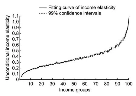
Fig.2 Unconditional income elasticities in 100 income groups.Group 1 is the lowest income group and Group 100 is the highest income group. Source:Calculated based on the NBSC(National Bureau of Statistics of China) household survey data used in this study.

The simulated results of possible trends of beef consumption calculated by eq.(14) in two mediumgrowth scenarios (S3 and S4) are presented in Fig.3,and the simulation results of two high-growth scenarios(S1 and S2) and two low-growth scenarios (S5 and S6)are displayed in Figs.4 and 5,respectively. Obviously,the simulation results show strong evidence that China’s beef consumption could expand rapidly with income growth,which might be underestimated if the difference in income elasticity across income groups is not taken into consideration.

In the medium-growth scenarios in Fig.3,the S3 scenario shows that beef consumption is expected to increase by 23.7% in the following 10 years and by 39.5%in the following 15 years when diverse income elasticities in 100 income groups were considered. Without considering the diverse income elasticities in the S4 scenario,beef consumption might be underestimated by 4.1 percentage points after a 10-year income increase. It is remarkable that the underestimation would widen over time. As a result,after a 15-year income increase,beef consumption is underestimated by 10.2 percentage points.

According to Figs.4 and 5,the results of S1 and S5 provide evidence that beef consumption would increase by 38.8 and 12.0%,respectively,in the following 10 years in the high-and low-growth scenarios with different income elasticities across 100 income groups. In addition,the 15-year income growth might lead to an increase in beef consumption by 70.5 and 18.6% in the high-and low-growth scenarios,respectively. Furthermore,without considering the diverse income elasticities in S2 and S6 scenarios,beef consumption could be underestimated by 27.2 and 1.5 percentage points after a 15-year income increase,respectively.

Table 4 Result of robust analysis

Table 5 Simulation scenarios

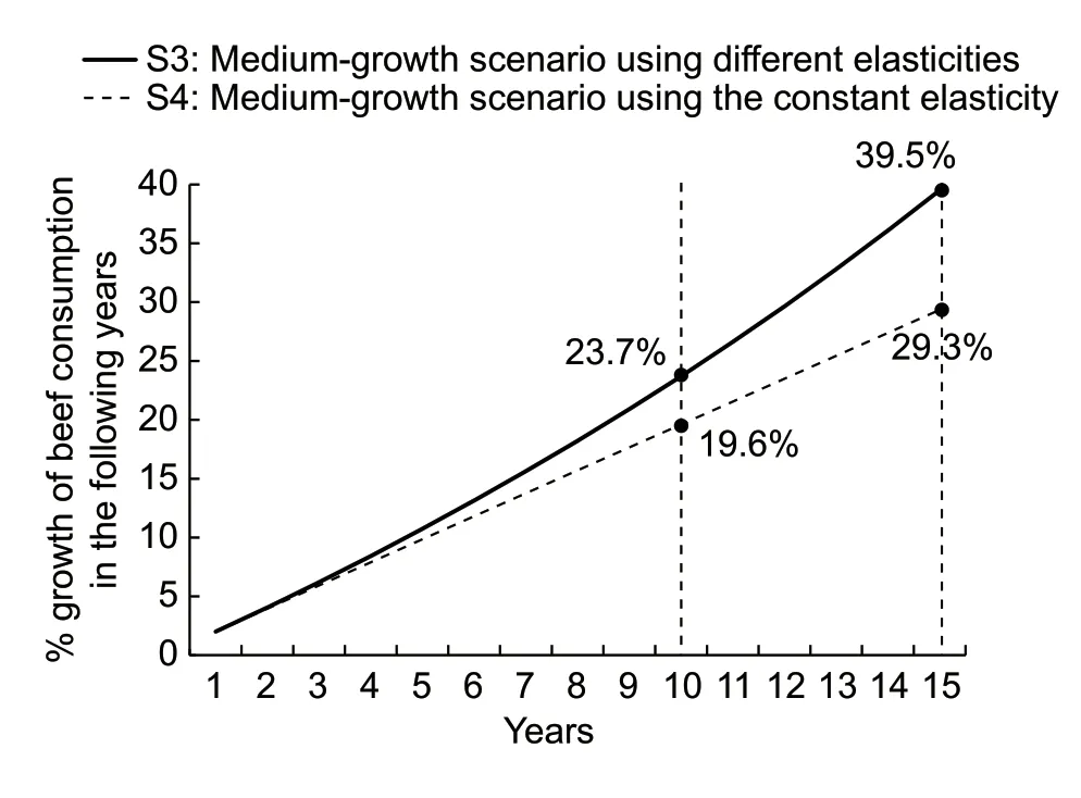
Fig.3 Increase in beef consumption in medium-growth scenarios. Source:Calculated by using eq.(14) and based on the NBSC (National Bureau of Statistics of China) household survey data used in this study.

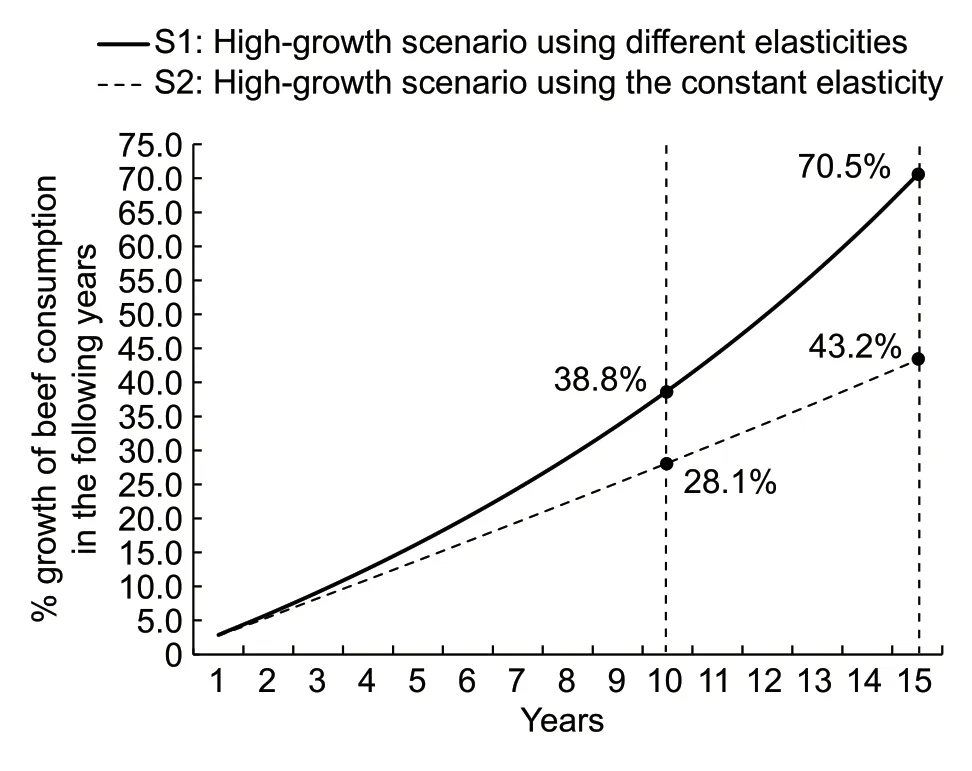
Fig.4 Increase in beef consumption in high-growth scenarios.Source:Calculated by using eq.(14) and based on the NBSC(National Bureau of Statistics of China) household survey data used in this study.

To enhance the credibility of the simulation results,we compared the simulation results considering the difference in income elasticity in this study (S1,S3,S5)with the research results ofOECD-FAO Agricultural Outlook 2019–2028that predicts the changes in China’s beef consumption by using a partial equilibrium model(OECD-FAO 2019). According to OECD-FAO (2019),on the one hand,China’s beef consumption could increase by 30.4% in the 15 years from 2009 to 2024,which is a little lower than the simulated result of S3 (39.5%) but within the growth interval of 18.6 to 70.5% simulated by low-,medium-and high-growth scenarios (S1,S3 and S5). On the other hand,OECD-FAO (2019) predicts that China’s beef consumption could increase by 24.2% in the 10 years from 2009 to 2019. This result is not only within the 10-year growth interval in S1,S3 and S5 (12.0–38.8%),but also very close to the S3 scenario (23.7%).

What requires explanation is that the perspective of the simulation section is to simulate the possible trends of beef consumption under income growth scenarios at the household level and analyze the impact of considering income elasticities of different income groups on the simulation results. Therefore,while our sample was collected between 2007 and 2009,the derived income elasticities for different income groups could still serve our purpose well in simulating the possible trend of beef consumption under different income growth scenarios.

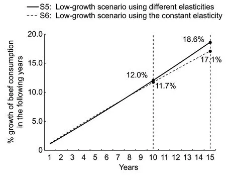
Fig.5 Increase in household beef consumption in low-growth scenario. Source:Calculated by using eq.(14) and based on the NBSC (National Bureau of Statistics of China) household survey data used in this study.

To further verify the robustness of the simulation results,we compared the trends of beef consumption of urban households living in cities with different levels of urbanization. The simulation results show that,the percentage growth of household beef consumption in large,middle and small cities are close to the results in the S3 scenario considering different income elasticities,which further enhances the reliability of the simulation results in this study. The detailed simulation results is presented in Appendix A. However,it should be noted that the simulation in this study is only a pilot analysis for possible trends of beef consumption and does not consider any consumption saturation point in the long run.

4.Discussion

In the short term,the global spread of COVID-19 may slow the growth of Chinese residents’ income to a certain extent (Zhanget al.2020). However,in the medium and long term,after the pandemic is contained,the beef consumption in China would increase with residents’rising income (Headey and Ruel 2020). Furthermore,Baiet al.(2020) finds that beef consumed away from home grows faster than their at-home counterparts,leading to further increase in beef demand in the future. Thus,it is vital to identify the potential trends of beef consumption in urban China. This provides insights as well as policy implications for the government and business stakeholders.

More to the point,ensuring steady and sufficient beef supply from multiple sources plays the most important role in meeting the expanding beef demand (Huanget al.2017). From the perspective of domestic production,it is necessary to increase the domestic supply capacity of safe and high-quality beef products for consumers,especially for those in the high-income groups who consume more beef and whose beef consumption grows faster with rising income than their low-income counterparts. To promote the production of beef and related products,China should urgently implement effective measures for the comprehensive development of its domestic beef industry,such as strengthening infrastructure construction,enhancing animal disease management as well as promoting technological innovation in the domestic beef supply chain.

Moreover,due to resource constraints and production efficiency different with other countries,China’s rising beef demand may have to partially depend on imports,which could lead to an increase in beef imports and benefit multinational beef business stakeholders,such as the beef producers in Australia,New Zealand,Argentina and other major beef exporters to China (OECD-FAO 2019). Therefore it is vital to diversity beef import sources to reduce import risks while minimizing import costs. In addition,in order to reduce import dependence,developing and strengthening domestic high-quality and well-known beef brands are also crucial.

5.Conclusion

This study estimates the income elasticities of beef demand across different income groups by using an IHS double-hurdle model and simulates the possible trends of beef consumption in urban China. Our most notable findings are as follows. First,the empirical results significantly indicate that the unconditional income elasticities of beef consumption at home are 0.385,0.169,0.353 and 0.671 for the full sample,low-,medium-,and high-income households,respectively. Second,our simulation results provide strong evidence that China’s beef consumption is expected to increase by 12.0–38.8%in 10 years and by 18.6–70.5% in 15 years under distinct income growth scenarios. But these could be underestimated if only one income elasticity for the whole population was considered.

Acknowledgements

This work was supported by the National Natural Science Foundation of China (71473251).

Declaration of competing interest

The authors declare that they have no conflict of interest.

Appendixassociated with this paper is available on http://www.ChinaAgriSci.com/V2/En/appendix.htm