Comparison between fluctuation of floating potential gradient and velocity of blob structure on HL-2A tokamak

Chenyu WANG (王晨宇), Lin NIE (聂林), Guixin TANG (唐圭新),Min XU (许敏), Rui KE (柯锐), Yihang CHEN (陈逸航),Huajie WANG (王华杰), Zhanhui WANG (王占辉), Shilin HU (胡世林), Ting WU (吴婷),Ting LONG(龙婷),Yuxuan ZHU(朱宇轩),Hao LIU(刘灏),3,Shaobo GONG(龚少博), Jinbang YUAN (袁金榜) and Longwen YAN (严龙文)

1 Southwestern Institute of Physics, Chengdu 610041, People’s Republic of China

2 Harbin Institute of Technology, Harbin 150001, People’s Republic of China

3 University of Science and Technology of China, Hefei 230026, People’s Republic of China

Abstract Several results based on the Langmuir probes’data on the HL-2A tokamak are presented.The blob structures’radial and poloidal drift velocities,estimated by the gradient of floating potential and by time delay evaluation, are compared in different line-averaged density and electron cyclotron resonance heating conditions.A positive correlation is observed in the comparison between blobs’radial velocity estimated by the two methods mentioned above, regardless of the situation differences mentioned above.Correlation is also observed in the comparison between the blobs’poloidal velocity estimated by the two methods in different situations, while a shift due to the different line-averaged density is observed.These results imply that the radial gradient of floating potential may have some value as a reference during data analysis in low-parameter discharge.

Keywords: Langmuir probe, blob structure, scrape-off layer

1.Introduction

In Langmuir probe diagnostics, the gradient of plasma potential is calculated by:

The first term on the right of equation (1) is the floating potential term,and the second one is the electron temperature term.In many experimental cases, due to reasons like the design or arrangement of the probes or the electrons’ bi-Maxwellian distribution [1, 2], it can be hard to obtain the electron temperature term of equation(1).A common solution is to use the floating potential term to estimate the gradient of plasma potential.Considering that the probe array normally provides the radial and poloidal message only, the approximation can be written as:

While the radial component of equation (2) is barely used due to the radial temperature gradient,which cannot be ignored,the poloidal component of equation (2) is widely used in many experimental data analysis cases.On HL-2A, the gradient of floating potential was used to estimate the blob’s radial velocity and further estimate the radial scale of the blob structure[3].On TEXTOR,the gradient of floating potential was used to estimate the radial velocity of the burst events and to evaluate the motion of these events[4].On T-10,the gradient was also used to define the poloidal field and to calculate the radial velocity; the radial velocity result showed that the blob structure on the device would move directly to the first wall[5].On ASDEX-U,the gradient of floating potential was used to estimate the electric field and to calculate the particle flux; it was found that during the ELM period, the outward flux would increase sharply [6].However,due to the arrangement of the probe array or for other reasons,there are still many cases in which the radial component of equation(2)needs to be used,such as estimating the shearing rate[7], calculating the Reynolds stress [8], or eddy measurement.

In order to determine whether the radial component of equation (2) could be used in some cases, the blob structure[9–16], which is generated in the edge of main plasma and driven by E×B drift, is studied.A fixed mid-plane probe array [17, 18] and a moving probe array is used to measure the radial and poloidal motions of blob structure during the low-parameter discharging of HL-2A.Based on the data of the probe arrays mentioned above, we try to compare the blob-induced fluctuation of floating potential gradient with the blob velocity measured by time delay evaluation (TDE).

In the next section, we show the experimental setup including the HL-2A discharging parameters, the scheme of probe array and the velocity calculation method.The results of data analysis are given in section 3, and finally, the conclusion and further discussion of the results are given in section 4.

2.Experimental setup

HL-2A is a medium-sized tokamak with major radiusR=1.65 m and minor radiusr=0.4 m [19].The current direction in HL-2A is counterclockwise while that of the toroidal magnetic field is clockwise.The probe diagnostic system on HL-2A[19]is located on the midplane of the tokamak,as shown in figure 1.The insertion speed is 1 m s−1while the extracting speed is about 0.5 m s−1.The probe can detect the plasma 3–4 cm inside the last closed flux surface (LCFS) under ohmic and L-mode discharges,and about 1 cm inside the LCFS under H mode.The sampling frequency is 1 MHz.

The experiment first uses a fixed 3×3 probe array,arranged as in figure 2(e),the radial position of which is fixed at 0.5 cm inside the LCFS on the midplane.This probe array is able to provide both the radial and poloidal velocity of the blob structures.The comparison of the radial velocity estimated by the poloidal gradient of floating potential and that estimated by the TDE method is regarded as a reference graph for the poloidal ones, since it is a consensus that the gradient estimation on poloidal direction is qualitatively right[20].For this reason, it can be predicted that the graph of these two radial velocities will be positively correlated.Besides, the comparison of poloidal velocity between the gradient estimation and TDE provides a large number of data points at the same radial position.

Second, a moving 3×3 probe array, arranged as in figure 2(f), is used.The approaching period of the Langmuir probe is about 80 ms.The data of this period are analyzed to compare the velocity estimated by the radial gradient of floating potential and TDE method at different radial positions.Since the blob structure is mainly observed and further developed in the scrape-off layer (SOL), only the results of different radial positions in the SOL are stated in this paper.

Figure 1.Arrangement of probe diagnostic system on HL-2A.

These 3×3 probe arrays are designed to comprise a three-stair array,as shown in figures 2(a)–(d).The stair height of the probe arraysdrbetween two adjacent probes, which is also the radial distance, is 2.5 mm, and the poloidal distancedθbetween two adjacent probes is 5 mm.The arrangement of the fixed probe is shown in figure 2(e)and the arrangement of the moving probe is shown in figure 2(f).

In figure 2(e), probesIs1–Is4are used to measure the ion saturation current at different radial/poloidal positions to estimate the blob velocity in the TDE method;Vf1–Vf4are used to measure the floating potential at different radial/poloidal positions to calculate the floating potential gradient in both the radial and poloidal directions.In the case of the fixed probe,the gradient of floating potential is calculated as:

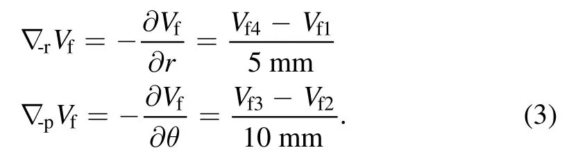
Terms ∇‐rVfand ∇‐pVfare the values of the negative radial/poloidal gradient of floating potential inside the blob.

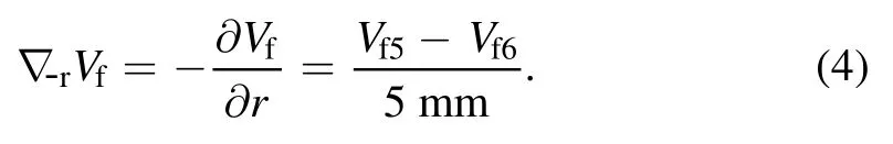
In figure 2(f), probesIs5andIs6are used to estimate the blob’s poloidal velocity by TDE,while probesVf5andVf6are used to measure the floating potential at different radial positions and to calculate the gradient of floating potential.In the moving probe case, term ∇‐rVfbecomes:

3.Experimental results

3.1.Discharging parameter

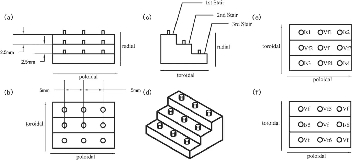
Figure 2.Arrangement of the three-stair probe array.(a)–(d)Design and basic parameters of the three-stair probe array,(e)probe arrangement for the fixed probe, and (f) probe arrangement for the moving probe.

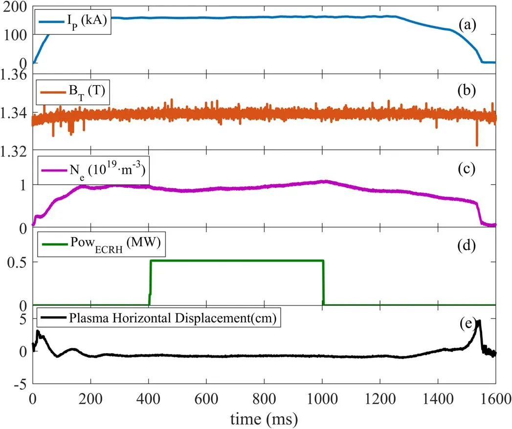
Figure 3.Discharging parameter evolutions of (a) the plasma current, (b) the toroidal magnetic field, (c) the line-averaged electron density,(d) the power of ECRH, and (e) the plasma horizontal displacement.

Both experiments were carried out under similar discharging parameters.Figure 3 shows the time evolution of typical parameters for a low-parameter discharge.From the top to the bottom are:(a)the plasma currentIP=150 kA;(b)the toroidal magnetic feildBT=1.34 T;(c) the line-averaged electron densityne～1.0 ×1019m−3; (d) the power of electron cyclotron resonance heating(ECRH)PECRH=0.5 MW;(e)the plasma horizontal displacementdh～0 cm.

Figure 4.Profiles of electron density (a) and temperature (b).

The profiles of electron density and temperature during low-parameter discharging are shown in figure 4, measured by a typical midplane reciprocating triple probe.From 65 mm outside the LCFS to ～15 mm inside the LCFS, the density and temperature slowly increase from ～0.5 ×1018m−3and 10 eV at 25 mm to ～4×1018m−3and 40 eV; the maximum gradient of density is ～5×1019m−4,and the maximum gradient of electron temperature is ～1000 eV m−1.

The effect of the discharging parameter—to be specific,the line-averaged density and the ECRH condition—on the blob’s drift velocity is observed in the experimental results,and demonstrated in section 3.3.

3.2.Velocity calculation

The fixed probe experiment measured the blobs in the midplane,the radial position of which is ～5 mm inside the LCFS,while the moving probe experiment measured the blobs in the midplane with different radial positions in the SOL.The characteristic signals were obtained by the condition average(CA)method[21–24].This method can extract structure from turbulence based on a preset amplitude thresholdδnedefined as the perturbation of electron densityne,which is calculated byne−〈ne〉 ,where the brackets〈...〉 denote the time average.In the fixed probe experiment, the threshold was preset asδne=2.5σwhereσis the standard deviation ofne.A previous study [3] showed that with thresholdδne/σ=2.5the statistical characterizations of the blobs’ radial size and poloidal size were ～20 mm, which is larger than the radial distance(dr=5 mm)and poloidal distance(dθ=10 mm)of the 3×3 probes.In the moving probe experiment, the threshold was set toδne=1.5σin order to obtain more blob cases.The size of the blob estimated by the TDE method was still about 15–20 mm,which is also larger than both the radial and poloidal distances.Combined with the CA method, the radial/poloidal velocities and floating potential gradients of the blobs can be calculated.

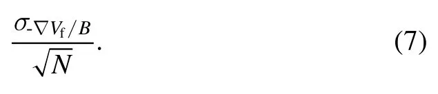
Based on the CA result shown in figure 5 and the parameter provided by the figure, the velocity can be estimated.For the fixed probe,the radial velocity can be estimated by the following equation:

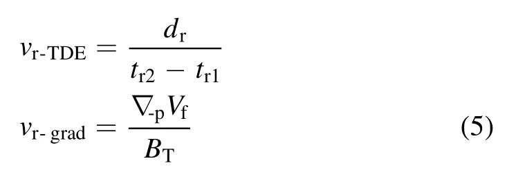
vr‐TDEandvr‐gradin equation (5) are the radial velocity estimated by TDE and the radial velocity estimated by the gradient of floating potential, respectively.Termstr1andtr2are the times when the CA results of(Is1+Is2)/2and(Is3+Is4)/2reach the peak values, and term ∇‐pVfhere r epresents the peak value of(Vf3−Vf2)/dθ.

Similarly, for both the fixed and moving probes, the poloidal velocity can be estimated as:

vp‐TDEandvp‐gradin equation (6) are the poloidal velocity estimated by TDE and the poloidal velocity estimated by the gradient of floating potential, respectively.Termstp1andtp2are the time when the CA results of(Is2+Is4)/2and(Is1+Is3)/2for the fixed probe, andIs5andIs6for moving probe reach the peak values in sequence.The term ∇‐rVfhere denotes the peak value of(Vf4−Vf1) /drfor the fixed probe and(Vf5−Vf6)/drfor the moving probe.

Based on the two velocity estimation methods, the error bar of the estimating value is given below.The error bar of the velocity estimated by the gradient of floating potential is given as

Termσ‐∇Vf/Bis the standard deviation of all the single blobs’velocities in the selected time period, and termNrepresents the number of blobs in the selected time period, which is normally about 40–70 blobs in this paper.

In the TDE method, the time resolution of time delay Δtr/p=tr/p2−tr/p1is dependent on the sampling frequency of the diagnostic system; since the sampling frequency of the probe is 1 MHz, the time resolution is 10−6s.Thus,the error range of the time delay is± 10−6ms,and the upper and lower error bars of the velocity estimated by the TDE method aredr/p[ 1(Δtr/p−10−6)−1(Δtr/p)]anddr/p[ 1(Δtr/p) −1(Δtr/p+10−6)], respectively, in units of m s−1.

3.3.Result comp arison

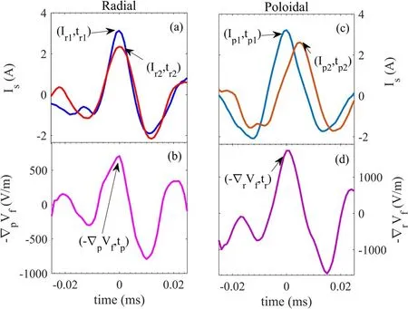
Figure 5.Velocity estimation:(a)radial velocity estimated by TDE,(b)radial velocity estimated by the negative gradient of floating potential,(c) poloidal velocity estimated by TDE, and (d) poloidal velocity estimated by the negative gradient of floating potential.

Figure 6.Radial velocity comparison results under different discharging conditions at the radial position of 0.5 cm inside the LCFS.

As mentioned in section 2, the comparison of the radial velocity is given first as a reference graph for the following poloidal velocity comparison graphs.The radial velocity comparison result based on the analysis of the fixed probe is shown in figure 6.Thexaxis represents the TDE-estimated velocity while theyaxis represents the floating potential gradient-estimated velocity.As predicted before,the gradientestimated radial velocity and the TDE-estimated radial velocity are positively correlated.Based on a brief linear fit,the slope of figure 6 is around 1 and the linear fit result passes point(0,0).In addition,in figure 6,the data are marked with different tokens by their discharging parameters.As shown in figure 6, data under the same discharging condition are congregated in very similar areas: the group marked by red crosses with line-averaged density1.5 ×1019m−3and 0.5 MW ECRH is congregated in the bottom left part of the figure,while the group marked by green diamonds,which has the same line-averaged density as red cross group but the ECRH removed, is congregated in the center of the figure.Thus, it can be concluded that, under the same discharging conditions other than the ECRH, the absence of ECRH leads to an increase in the drift velocity estimated by both methods,which is a predicted result as well.Finally,the group marked by blue circles, for which the line-averaged density is 1.0 ×1019m−3and the power of ECRH is 0.5 MW, is congregated in the top right part of the figure.It can be observed in figure 6 that the overall data,as well as the data inside each separated group, are all linearly correlated, and the slope of these overall data seems to be very similar to the slope of each individual group.

At the same radial position, the graphs of the velocity estimated by the two different methods are somehow different to figure 6.As shown in figure 7, though the velocity estimated by the two methods is still linearly correlated inside the three independent groups, and all three groups seem to share the same slope of about 1.2,a shift caused by the difference in line-averaged density can be observed.Moreover, while the two groups with line-averaged density of 1.5 ×1019m−3are distributed along the same straight line with a slope of 1.2,these two groups are clearly separated from each other,just as in figure 6.The group with 0.5 MW ECRH is congregated in the bottom left part of the figure and the group without ECRH is congregated in the top right part.This means that when the ECRH is absent, the velocity estimated by both methods is increased dramatically, which gives us indirect support of stating the reference value of estimating the radial gradient of plasma potential by the gradient of floating potential.A possible explanation for the difference between the graphs in figures 6 and 7 is related to the characteristic of the blob structure itself.In the radial–poloidal section, the structure is ambipolar due to the charge separation in the poloidal direction, which is caused by the curvature of the magnetic field.Thus,when estimating the internal poloidal field by two separate probes, the result is close to the one given by the TDE method.For the same reason,when estimating the radial component of the internal electric field, the two separated probes are in a direction almost perpendicular to the internal electric field, so an erroneous result is given, and that is the reason why there is a large discrepancy between the velocity estimated by the gradient of floating potential and the velocity estimated by the TDE method.Besides,the local electric field is very sensitive to the local charge fluctuation, and thus an increased density may lead to an increase in the error, which could explain the shift that occurs in figure 7.

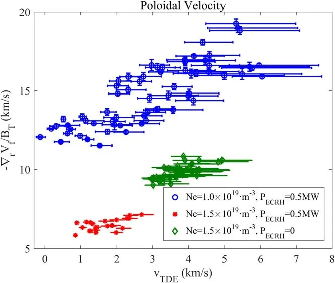
Figure 7.Comparison of poloidal velocity under different discharging conditions at the position 0.5 cm inside the LCFS.

In addition, by analyzing the data from the movable probes,the poloidal velocity estimated by the two methods at different radial positions is exhibited in figure 8.It is observed that in different radial positions in the SOL, from 5–6 cm outside the LCFS to 1–2 cm outside the LCFS, the gradientestimated velocity and TDE-estimated velocity show a positive correlation in the graph.Moreover, the amplitude of the velocity does not vary a lot from position to position, which implies that the blob’s velocity does not change much in the SOL.Compared with figure 7, though the fitting function of figure 8 is still a linear function, the slope of the fitted function is notably lower than 1 at only about 0.1.The reason for the slope difference might be the radial position, since figure 7 is based on the data inside the LCFS, while figure 8 shows the data outside the LCFS,and thus the slope could be different due to the different plasma environment.Just as mentioned before,even in the SOL,the two separated probes lie on a line that is almost perpendicular to the local electric field, so there is an error.In addition, the density difference between the edge plasma and SOL plasma is significant.

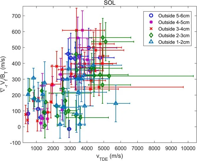
Figure 8.Poloidal velocity in different radial positions in the SOL.

Therefore, this might be an explanation why the slope changed a lot and why the velocity estimated by the gradient of floating potential decreased a lot.

4.Conclusion and discussion

The poloidal velocity graphs of both the fixed probe (see figure 7)and the moving probe(figure 8)showed similarity to the reference graph (figure 6), which is the graph of radial velocity estimated by the two methods.It can be implied that under low-parameter discharging, in the edge and SOL regions,using the gradient of floating potential to estimate the plasma potential ones is qualitatively accurate.

To discuss why this estimation is qualitatively right, some reasons are given.Figure 9 gives the CA result of the radial gradient of floating potential and the radial gradient of electron temperature, which are the two parts of the gradient of plasma potential,with different preset thresholds fromσ2 toσ3.5 at the relative radial position inside LCFS ～0.5 cm,very similar to the fixed probe’s radial position.It is observed that though there is a phase difference between the results in figures 9(a) and (b), as the threshold becomes higher,both the amplitude of the gradient of floating potential and the gradient of electron temperature increase.This could provide a possible explanation for the results in figures 7 and 8: as the radial gradient of plasma goes up, the radial gradients of floating potential and electron temperature go up.In this situation,though the effect of the electron temperature term in equation (1) cannot be ignored, as the poloidal gradient estimation usually assumes,the radial gradients of floating potential and electron temperature are still positively correlated.

Further support is given by the comparison of the CA results of the radial gradients of floating potential and electron temperature.The reference signal is the ion saturation current,and the preset threshold is 2.5σ.The graph is given in figure 9(c).As shown in figure 9(c), the peak values of the radial gradients of floating potential and plasma potential are positively correlated.Thus, in some cases, the effect of the temperature term in equation (1) can be neglected.

Figure 9.(a)CA result of radial gradient of floating potential with different thresholds,(b)electron temperature with different thresholds,and(c) comparison of the peak values of CA results.

Acknowledgments

This research is supported by the National Key Research and Development Program of China (Nos.2017YFE0300500,2017YFE0300501) and No.2018YFE0309100 and National Natural Science Foundation of China (Nos.11705052,11875124, 11905050, 11875020 and U1867222).

ORCID iDs

Chenyu WANG (王晨宇) https://orcid.org/0000-0001-5318-7380