Flexible rotation of transverse optical field for 2D self-accelerating beams with a designated trajectory

Lei Zhu, Xuesong Zhao, Chen Liu, Songnian Fu, Yuncai Wang and Yuwen Qin

Keywords: self-accelerating beams; optical field; caustic

Introduction

Self-accelerating beams are the solutions to the wave equation, with intensity peak traveling along a curved trajectory during the free-space propagation1. The concept of snake beams has been proposed by Rosen and Yariv in 19952. However, it was until 2007 that Siviloglou and Christodoulides first experimentally generated the Airy beam with a parabolic trajectory3,4. Self-accelerating beams have attracted worldwide attentions in the field of high-resolution imaging5, particle manipulation6,light bullets7,8, micro-machining9, and obstacle evasion optical communication10,11. Self-accelerating beams also have broad and important applications beyond optics,due to the similar form of wave equations, so that self-accelerating beams can be easily introduced into acoustic waves12, electronic waves13, and plasmonic waves14−16.

Generally, the main lobe of self-accelerating beams possesses most energy of transverse optical field and propagates along a curved trajectory. Consequently, previous research works and applications were mainly focused on the main lobe of self-accelerating beams. For practical applications, self-accelerating beams with flexible trajectory manipulation are required. One way is to find other analytical solutions to the wave equation, such as Bessel-like self-accelerating beam with circle trajectory17, Mathieu beam with elliptical trajectory18, and Weber beam with parabolic trajectory19. However, an efficient strategy to generate the accelerating beam with an arbitrary trajectory is to use the optical caustic strategy20,21, even though the generated beam is not the exact accelerating non-diffraction solution to the wave equation. The caustic method was first proposed by Greenfield in 201122, then it has been extended from paraxial beams to non-paraxial beams18,19in order to obtain large bending angle, and from the convex trajectory to non-convex trajectory23,24. However, unlike Gaussian beam or Bessel beam, since the light rays have to be distributed outside the local convex part of the trajectory according to the optical caustic, the transverse optical field of 2D self-accelerating beams with a curved trajectory is definitely not circularly symmetrical around the main lobe. For example, the transverse optical field of 2D Airy beam is mainly located at a quarter of the transverse plane. Such asymmetrical distribution of side lobes has to be taken into account, when 2D self-accelerating beams are involved for some optical field distribution sensitive applications, such as micro-machining, particle manipulation, and free-space photonic interconnection.Although the transverse rotation of optical field for 2D self-accelerating beams can be realized by loading a rotated phase pattern into the spatial light modulator(SLM), the corresponding trajectory varies as well. Such a solution may not be ideal for some practical applications, because the main lobe possesses the most energy of 2D self-accelerating beams, and the trajectory of main lobe has to be maintained as well. Therefore, flexible manipulation of transverse optical field without changing the designated trajectory is highly desired.

In this submission, we firstly identify that the transverse optical field is closely associated with the selection of transverse Cartesian coordinates, when 2D self-accelerating beams are generated by the optical caustic method. Consequently, we propose a coordinate-rotation based strategy, in order to realize optical field rotation within 90 degrees. Finally, a proof-of-concept experiment to verify our proposed method is demonstrated for the application of obstacle evasion free-space photonics interconnection.

Operation principle of manipulating transverse field distribution

Generally, the free-space propagation of optical field can be expressed as the integral of angular spectrum diffraction

whereA(kx) andϕ(kx) are the amplitude and phase distribution of the initial angular spectrum,kdenotes the wavenumber, andkxis the wavenumber inXdirection.Applying the stationary-phase approximation22,25to the integral, the main contribution toE(X,Z) comes from the stationary points where

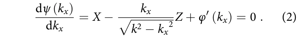
For a specific spatial frequencykx, Eq. (2) indicates that the stationary points are along a straight line. As a result, the propagation behavior of optical field can be simplified by a series of light rays, which can be analyzed by geometric optics. Besides, from the view of real space22, applying the stationary-phase approximation to the Fresnel diffraction integral, we can obtain the same conclusion.

The bending trajectory of self-accelerating beams can be explained by the caustic phenomenon, where the light rays are tangent to the bending trajectory, instead of being focused to a specific point. Consequently, in order to realize a self-accelerating beam with an arbitrary trajectory, we can first get a family of light rays which are tangent to the desired trajectory, then back-trace them to obtain the initial optical field or its spatial spectrum.Since the light rays are tangent to the trajectory, they have to be distributed at the convex side of the trajectory.Meanwhile, 2D self-accelerating beam can be regarded as the combination of two 1D self-accelerating beams in planes of (X,0,Z) and ( 0,Y,Z). As shown in Fig. 1, 2D self-accelerating beam with a convex trajectory is taken as an example. The projection of the curved trajectory on the initial plane is highlighted as a red curve in Figs. 1(c)and 1(f). With the trajectory decomposed into planes of(X,0,Z) and (0,Y,Z), theXandYcomponents of trajectory and light rays are shown as red curves and blue light rays in Figs. 1(a) and 1(b), respectively. As we can see, the light rays are located at the positive direction ofXaxis and the negative position ofYdirection. Hence,the corresponding optical field of pointAin the default Cartesian coordinates is shown as the blue area of Fig. 1(c). However, under the condition of the fixed freespace trajectory, it can be decomposed to different coordinate pairs. Based on the new coordinates which are rotated counterclockwise with an angle ofθfrom the initial one, the components of the trajectory and light rays vary, as shown in Figs. 1(d) and 1(e). Accordingly, the optical field distribution is coordinate-dependent and can be rotated with an angle ofθ, as shown in Fig. 1(f).Therefore, we can conclude that the transverse optical field is associated with the selection of the transverse Cartesian coordinates, when 2D self-accelerating beams are generated by composing two independent 1D self-accelerating beams.

Fig. 1 | Generation of 2D self-accelerating beam based on optical caustic and the rotation principle of transverse optical field for 2D self-accelerating beam. Two perpendicular components (a)−(b) of trajectory and light rays in default Cartesian coordinates. (c) The projection of multiplexed trajectory and the distribution of transverse optical field in default Cartesian coordinates; two perpendicular components (d)−(e) of trajectory and light rays in rotated Cartesian coordinates. (f) The projection of multiplexed trajectory and the rotated distribution of transverse optical field in rotated Cartesian coordinates.

Simulation results and experimental verifications

In order to verify the coordinate-dependent optical field distribution, an experimental characterization setup is schematically shown in Fig. 2. At the output of standard single mode fiber, the light beam from a distributed feedback (DFB) laser at operation wavelength of 1550 nm is collimated to a Gaussian beam with a waist radius of about 1.75 mm. After passing through a linear polarizer(P) and a beam splitter (BS), the beam is spatially modulated by a reflective SLM (PLUTO-TEL-013, HOLOEYE)with a resolution of 1920×1080 and a pixel pitch of 8 μm.Fourier modulation is utilized in order to generate highquality 2D self-accelerating beams, in comparison with the real-space modulation. Therefore, a lens with a focal length of 0.2 m is set after the SLM, and the 2D self-accelerating beams can be obtained behind the lens.

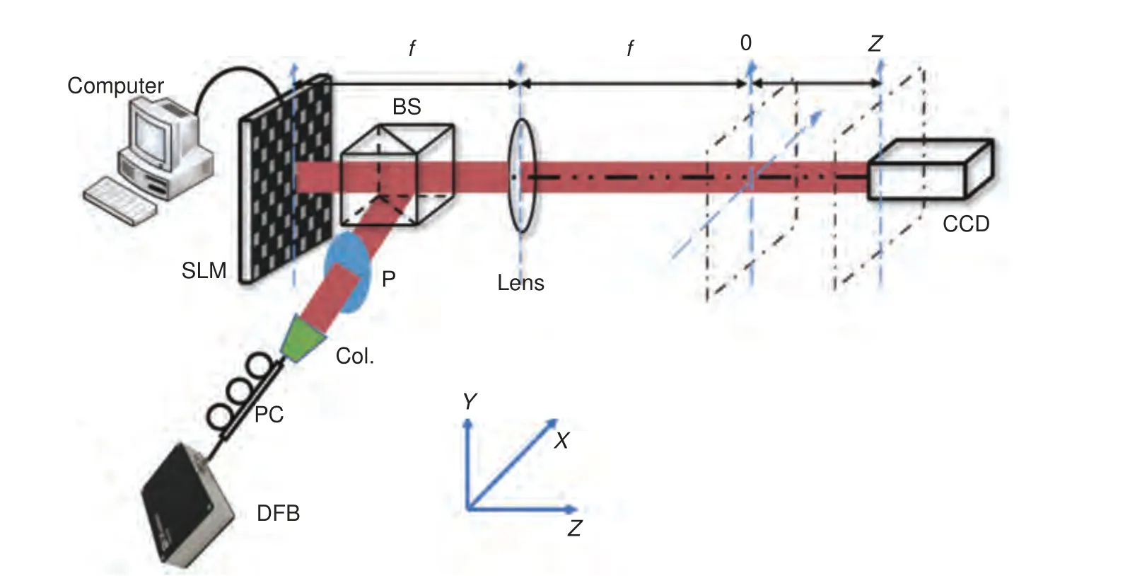
Fig. 2 | Experimental setup for the optical field rotation of 2D self-accelerating beams. DFB: distributed feedback laser; Col.: collimator; PC:polarizer controller; P: polarizer; BS: beam splitter; SLM: spatial light modulator.

Phase pattern

Generally, there are two approaches to generate self-accelerating beams, including Fourier space modulation with the help of a lens and real space modulation. Our experimental setup is based on the spatial spectrum modulation in Fourier space. Both two approaches can be unified in the phase space26by the Wigner distribution function (WDF)27. The physical meaning of WDF in optics can be approximately interpreted as the intensity of a light ray with a specific position and direction. We discuss the general curved trajectory with the form ofX=f(Z),Y=g(Z). After two orthogonal coordinates are rotated anticlockwise with an angle ofθ, the designated trajectory under the new coordinates is

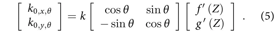
Since the light rays are tangent to the designated trajectory, after the coordinate rotation, emitting positions of light rays from the initial plane (planeZ=0) can be obtained as

and the direction of each light ray is

Next, according the reference26, the WDF of initial optical field can be expressed as

wherexθandyθdenote the coordinate variables of the initial plane (Xθ,Yθ,0). The phase pattern to be loaded on the SLM is determined by the phase distribution of the calculated optical field at the initial plane, which can be obtained according to the properties of WDF26,

where, for a lens-based Fourier transformation system,kx,θ=2πxθ/(λf),ky,θ=2πyθ/(λf),fis the focal length of lens. Due to the relationships in the right-hand coordinate system includingxθ+90°=yθ,yθ+90°=−xθ,x0,θ+90°=y0,θandy0,θ+90°=−x0,θ, we can derive

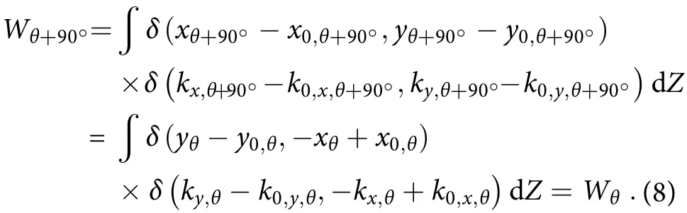
It indicates that the Wigner distribution function for our scheme varies with a period of 9 0°. Then, we can further obtainϕθ+90°=ϕθ. Therefore, the phase patterns for the transverse field with rotation angles ofθ+90°andθare identical. As a result, the transverse optical field can rotate within 90°while the trajectory is maintained without the modification. Since the light rays have to be located at the convex part of the trajectory, the range of rotation angle cannot exceed 90°with our proposed method.

Simulation results

As a typical self-accelerating beam with the convex trajectory, 2D Airy beam4is selected to verify the proposed optical field rotation technique. We set the trajectory of 2D Airy beam as

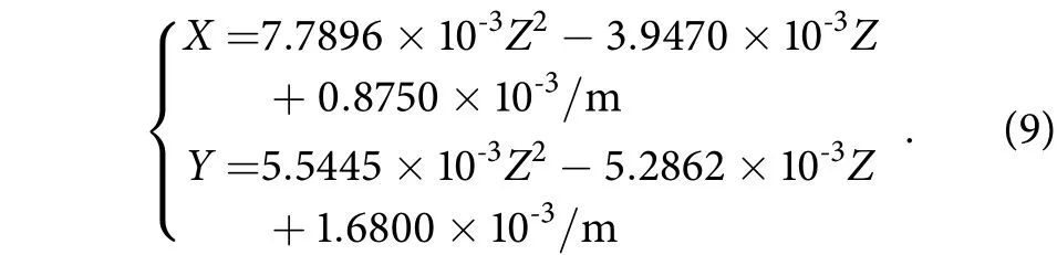
The original phase pattern in the default Cartesian coordinates, is shown as Fig. 3 (a). The corresponding 3D optical field distribution is calculated in Fig. 3(b), and the red curve denotes the trajectory. The projection of trajectory is shown in Fig. 3(c), which is consistent with Eq.(9). From Fig. 3(b), we can find that the boundary lines of transverse optical field are parallel to theXandYaxis,and the optical field is mainly distributed within this right-angle area. If the rotation of optical distribution is desired, a straightforward way is to simply rotate the phase pattern in the default Cartesian coordinates around its center with the specific angle, like in Fig.3 (d)with phase pattern rotation angle of -3 0°. The calculated 3D optical distribution of beam generated by the rotated phase pattern is shown as Fig. 3(e). The optical field distribution is rotated with an angle of -3 0°. However, the trajectory is rotated aroundZaxis as well, as shown in Fig. 3(f), which is not preferred. On the contrary, with the re-calculated phase patterns by our proposed method, as shown in Figs. 3(g) and 3(j), the optical distribution is rotated with an angle of -3 0°and 15°, and the trajectory can be maintained without the modification, as shown in Figs. 3(h), 3(i), 3(k) and 3(l).

Experimental results

The phase patterns to be loaded on the SLM for generating the 2D Airy beams with rotation angles of-30°,0°and 15°are calculated, respectively, according to Eq. (6)and (7), as shown in Figs. 4(a−c). The white dotted lines in Figs. 4(d−u) are the projection of the designated trajectory on the initial plane. The intensity profiles are captured every 5 cm from the back focal plane of lens, but only the results at distance of 0, 0.3 m and 0.6 m are presented here. In Fig. 4, we find the experimental results are in good agreement with our simulation results.The main lobes of the experimentally generated light beams at distance of 0.3 m are precisely located at the white dotted projection of trajectory, but there occur few deviations at distance of 0 and 0.6 m. We infer that the optical path is not fully aligned. However, we can conclude that the transverse optical field of 2D Airy beams generated in our experiments can be successfully rotated in a manageable way.

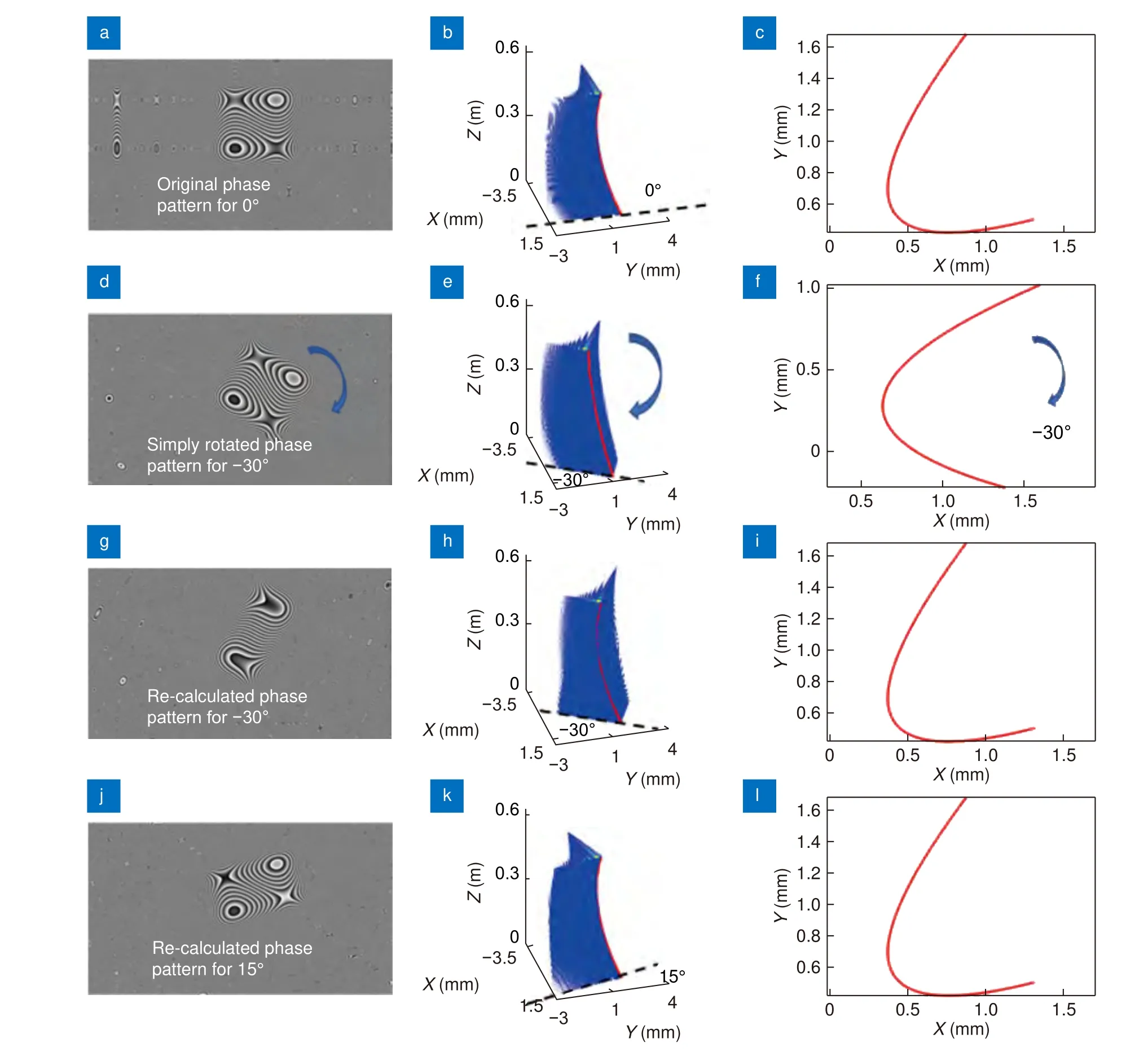
Fig. 3 | Different phase patterns and their calculated 3D optical distribution and trajectories. (a) Original phase pattern and its (b) 3D optical distribution and (c) the projection of trajectory. (d) Simply rotated phase pattern for -30° and corresponding (e) 3D optical distribution and (f)the projection of trajectory. (g), (j) Re-calculated phase patterns for -30° and 15°, and (h), (k) their 3D optical distribution and (i), (l) the projection of trajectory.

Application of free-space photonic interconnection

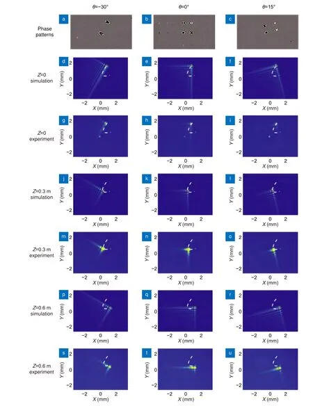
Fig. 4 | Calculated and experimental results for the optical field rotation of 2D Airy beam at different propagation distances. (a − c) Calculated phase patterns. (d − f), (j − l), (p − r) Simulated and (g − i), (m − o), (s − u) experimental intensity profiles at distance of 0, 0.3 m and 0.6 m with a rotation angle of -30°, 0° and 15°, respectively.

When an obstacle occurs at the light path of free-space photonic interconnection system, the interruption happens. Therefore, a curved trajectory of 2D self-accelerating beams is helpful to realize the obstacle evasion photonic interconnection, because the appropriate trajectory of 2D self-accelerating beams can be designed to evade the obstacle. We assume that the positions of transmitter and receiver are atT(0,0,0) andR(0,0,0.6 m),respectively. A thin opaque circle obstacle with its quarter removed, whose center is put at the position ofC(1 mm, 1 mm, 0.3 m), is set at the distance of 0.3 m, as shown in Fig. 5(a). PointOdenotes the intersection ofZaxis and obstacle plane. The obstacle can be rotated around its center pointCfreely along the vertical dotted line with an angle ofβ. To evade the obstacle, the trajectory of 2D Airy beam must pass through pointsT,CandRsuccessively. The trajectory of 2D Airy beam is set asX=Y=−11.4305×10-3Z2+6.8583×10-3Z/m, as shown in the red parabolic curve of Fig. 5(a). Under such a trajectory,the main lobe of 2D Airy beam is able to bypass the obstacle and be successfully collected by the receiver. If the optical field of the generated beam is fixed, the bypassed energy is different when the obstacle anglesβare varied. Therefore, the bypassed energy can be optimized by the selection of 2D Airy beam with an appropriate optical field distribution. The 2D Airy beam with the rotated optical field is generated with an angle ofθfrom-45°to 4 5°. Meanwhile, the obstacle is experimentally rotated withβ=-15°,0°and 3 0°, respectively. After the obstacle, another lens is used to converge the bypassed light to a small spot and an integral sphere is used to collect the bypassed optical energy. The calculated results together with the experimental measurements after the normalization are shown in Figs. 5(b−d). Due to the non-fully aligned optical axis and mechanical variation,it is challenging to set the main lobe of Airy beam atz=0.3 m locate at pointCprecisely when the obstacle is rotated. The position deviation between main lobe and pointCleads to some transmittance differences between the simulation and experimental results. However, it is clearly observed that, when the rotation angles of obstacle and the optical field are identical, the bypassed optical power can approach the maximum value. Consequently, after we design an appropriate trajectory to evade obstacle, the interconnection performance can be further optimized when the obstacle structure and the corresponding optical field distribution are simultaneously taken into consideration.

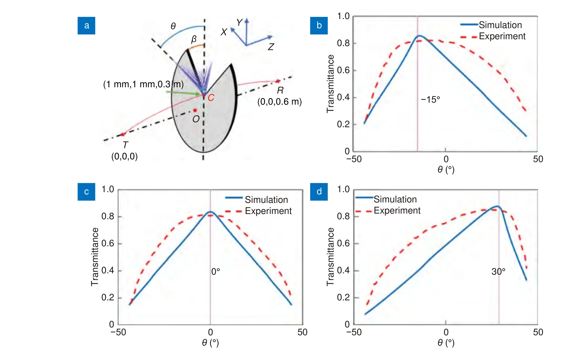
Fig. 5 | Obstacle evasion experiment. (a) set-up; normalized received optical power with obstacle’s angle β of (b) -15° (c) 0° and (d) 30°. (blue solid curves are calculated results, and red dotted curves denote the experimental results.)

Conclusions

We have demonstrated a scheme to realize a flexible rotation of transverse field for 2D self-accelerating beams under the condition of a fixed trajectory. Based on the rotation of transverse Cartesian coordinates, the transverse optical field can be flexibly rotated within 90 degrees. By selecting 2D Airy beam as a simple 2D self-accelerating beam with a single convex trajectory, we verify the scheme numerically and experimentally. Since the operation principle of the proposed method is based on the caustic analysis, it can apply to other self-accelerating beams. The proposed scheme to flexibly manipulate the rotation of transverse optical field is helpful for some applications sensitive to the optical field distribution for 2D self-accelerating beams, such as optical tweezers and laser micro-machining.

Acknowledgements

We are grateful for financial supports from National Key R&D Program of China (Grant No. 2018YFB1801001), the National Natural Science Foundation of China (Grant No. 61875061), and the Program for Guangdong Introducing Innovative and Entrepreneurial Teams.

Competing interests

The authors declare no competing financial interests.