Relationship between manifold smoothness and adversarial vulnerability in deep learning with local errors∗

Zijian Jiang(蒋子健), Jianwen Zhou(周健文), and Haiping Huang(黄海平)

PMI Laboratory,School of Physics,Sun Yat-sen University,Guangzhou 510275,China

Keywords: neural networks,learning

1. Introduction

Artificial deep neural networks have achieved the stateof-the-art performances in many domains such as pattern recognition and even natural language processing.[1]However,deep neural networks suffer from adversarial attacks,[2,3]i.e., they can make an incorrect classification with high confidence when the input image is slightly modified yet maintaining its class label. In contrast, for humans and other animals,the decision making systems in the brain are quite robust to imperceptible pixel perturbations in the sensory inputs.[4]This immediately establishes a fundamental question: what is the origin of the adversarial vulnerability of artificial neural networks? To address this question, we can first gain some insights from recent experimental observations of biological neural networks.

A recent investigation of recorded population activity in the visual cortex of awake mice revealed a power law behavior in the principal component spectrum of the population responses,[5]i.e., the nthbiggest principal component (PC)variance scales as n−α,where α is the exponent of the power law. In this analysis, the exponent is always slightly greater than one for all input natural-image stimuli, reflecting an intrinsic property of a smooth coding in biological neural networks.It can be proved that when the exponent is smaller than 1+2/d,where d is the manifold dimension of the stimuli set,the neural coding manifold must be fractal,[5]and thus slightly modified inputs may cause extensive changes in the outputs.In other words, the encoding in a slow decay of population variances would capture fine details of sensory inputs, rather than an abstract concept summarizing the inputs. For a fast decay case,the population coding occurs in a smooth and differentiable manifold,and the dominant variance in the eigenspectrum captures key features of the object identity. Thus,the coding is robust, even under adversarial attacks. Inspired by this recent study, we ask whether the power-law behavior exists in the eigen-spectrum of the correlated hidden neural activity in deep neural networks. Our goal is to clarify the possible fundamental relationship between classification accuracy,the decay rate of activity variances, manifold dimensionality,and adversarial attacks of different nature.

Taking the trade-off between biological reality and theoretical analysis, we consider a special type of deep neural network, trained with a local cost function at each layer.[6]Moreover, this kind of training offers us the opportunity to look at the aforementioned fundamental relationship at each layer. The input signal is transferred by trainable feedforward weights,while the error is propagated back to adjust the feedforward weights via random quenched weights connecting the classifier at each layer. The learning is therefore guided by the target at each layer, and layered representations are created due to this hierarchical learning. These layered representations offer us the neural activity space for the study of the above fundamental relationship.

We remark the motivation and relevance of our model setting, i.e., deep supervised learning with local errors. As already known, the standard back propagation widely used in machine learning is not biologically plausible.[7]The algorithm has three unrealistic (in biological sense) assumptions:(i) errors are generated from the top layer and are thus nonlocal;(ii)a typical network is deep,thereby requiring a memory buffer for all layers’ activities; (iii) weight symmetry is assumed for both forward and backward passes. In our model setting,the errors are provided by local classifier modules and are thus local. Updating the forward weight needs only the neural state variable in the corresponding layer [see Eq. (2)],without requiring the whole memory buffer. And finally, the error is backpropagated through a fixed random projection,allowing easy implementation of breaking the weight symmetry.The learning algorithm in our paper thus bypasses the above three biological implausibilities.[6]Moreover, this model setting still allows a deep network to transform the low-level features at earlier layers into high-level abstract features at deeper layers.[6,8]Taken together,the model setting offers us the opportunity to look at the fundamental relationship between classification accuracy, the power-law decay rate of activity variances, manifold dimensionality, and adversarial vulnerability at each layer.

2. Model

where hi=δi,q(Kronecker delta function) and q is the digit label of the input image.

The local cost function Elis minimized when hi=Pifor every i. The minimization is achieved by the gradient decent method. The gradient of the local error with respect to the weight of the feedforward layer can be calculated by applying the chain rule,given by

After learning, the input ensemble can be transfered throughout the network in a layer-wise manner. Then, at each layer,the activity statistics can be analyzed by the eigenspectrum of the correlation matrix(or covariance matrix). We use principle component analysis (PCA) to obtain the eigenspectrum, which gives variances along orthogonal directions in the descending order. For each input image,the population output of nlneurons at the layer l can be thought of as a point in the nl-dimensional activation space. It then follows that,for k input images,the outputs can be seen as a cloud of k points.The PCA first finds the direction with a maximal variance of the cloud,then chooses the second direction orthogonal to the first one,and so on. Finally,the PCA identifies nlorthogonal directions and nlcorresponding variances. In our current setting,the nleigenvalues of the the covariance matrix of the neural manifold explain nlvariances. Arranging the nleigenvalues in the descending order leads to the eigen-spectrum whose behavior will be later analyzed in the next section.

3. Results and discussion

In this section,we apply our model to clarify the possible fundamental relationship between classification accuracy, the decay rate of activity variances,manifold dimensionality,and adversarial attacks of different nature.

3.1. Test error decreases with depth

We first show that the deep supervised learning in our current setting works. Figure 2 shows that the training error decreases as the test accuracy increases(before early stopping)during training. We remark that it is challenging to rigorously prove the convergence of the algorithm we used in this study,as the deep learning cost landscape is highly non-convex,and the learning dynamics is non-linear in nature. As a heuristic way,we judge the convergence by the stable error rate(in the global sense), which is also common in other deep learning systems. As the layer goes deeper, the test accuracy grows until saturation despite a slight deterioration. This behavior provides an ideal candidate of deep learning to investigate the emergent properties of the layered intermediate representations after learning,without and with adversarial attacks.Next, we will study in detail how the test accuracy is related to the power-law exponent,how the test accuracy is related to the attack strength,and how the dimensionality of the layered representation changes with the exponent, under zero, weak,and strong adversarial attacks.

Fig.2.Typical trajectories of training and test error rates versus training epoch. Lines indicate the train error rate, and the symbols are the test error rate. The network width of each layer is fixed to N =200 (except the input layer),with 60000 images for training and 10000 images for testing. The initial learning rate η =0.5 which is multiplied by 0.8 every ten epochs.

3.2. Power-law decay of dominant eigenvalues of the activity correlation matrix

A typical eigen-spectrum of our current deep learning model is given in Fig.3. Notice that the eigen-spectrum is displayed in the log–log scale,then the slope of the linear fit of the spectrum gives the power-law exponent α. We use the first ten PC components to estimate α but not all for the following two reasons: (i) A waterfall phenomenon appears at the position around the 10thdimension, which is more evident at higher layers. (ii)The first ten dimensions explain more than 95%of the total variance, and thus they capture the key information about the geometry of the representation manifold. The waterfall phenomenon in the eigen-spectrum can occur multiple times,especially for deeper layers[Fig.3(a)],which is distinct from that observed in biological neural networks[see the inset of Fig.3(a)]. This implies that the artificial deep networks may capture fine details of stimuli in a hierarchical manner. A typical example of obtaining the power-law exponent is shown in Fig.3(b)for the fifth layer. When the stimulus size k is chosen to be large enough (e.g., k ≥2000; k=3000 throughout the paper), the fluctuation of the estimated exponent due to stimulus selection can be neglected.

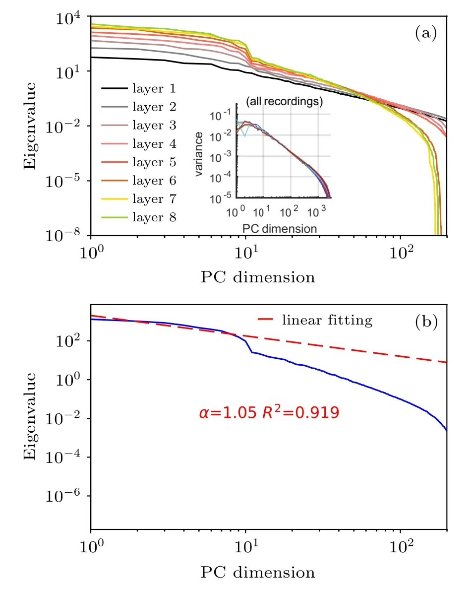
Fig.3. Eigen-spectrum of layer-dependent correlated activities and the power-law behavior of dominant PC dimensions. (a) The typical eigenspectrum of deep networks trained with local errors(L=8,N=200). Loglog scales are used. The inset is the eigen-spectrum measured in the visual cortex of mice(taken from Ref.[5]). (b)An example of extracting the power-law behavior at the fifth layer in(a). A linear fitting for the first ten PC components is shown in the log–log scale.

3.3. Effects of layer width on test accuracy and power-law exponent

We then explore the effects of the layer width on both test accuracy and power-law exponent. As shown in Fig.4(a),the test accuracy becomes more stable with increasing layer width.This is indicated by an example of nl=50 which shows a large fluctuation of the test accuracy especially at deeper layers. We conclude that a few hundreds of neurons at each layer are sufficient for an accurate learning.

The power-law exponent also shows a similar behavior;the estimated exponent shows less fluctuations as the layer width increases. This result also shows that the exponent grows with layers. The deeper the layer is,the larger the exponent becomes. A larger exponent suggests that the manifold is smoother,because the dominant variance decays fast,leaving few space for encoding the irrelevant features in the stimulus ensemble. This may highlight that the depth in hierarchical learning is important for capturing key characteristics of sensory inputs.

Fig.4. Effects of network width on test accuracy and power-law exponent α. (a) Test accuracy versus layer. Error bars are estimated over 20 independently training models. (b)α versus layer. Error bars are also estimated over 20 independently training models.

3.4. Relationship between test accuracy and power-law exponent

3.5. Properties of the model under black-box attacks

Fig.5. The power-law exponent α versus test accuracy of the manifold. α grows along the depth,while the test accuracy has a turnover at the layer 2,and then decreases by a very small margin. Error bars are estimated over 50 independently training models.

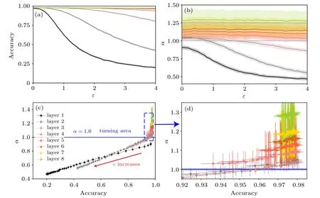
Fig.6. Relationship between test accuracy and power-law exponent α when the input test data is attacked by independent Gaussian white noises.Error bars are estimated over 20 independently training models. (a) Accuracy versus ε. ε is the attack amplitude. (b) α versus ε. (c) Accuracy versus α over different values of ε. Different symbol colors refer to different layers. The red arrow points to the direction along which ε increases from 0.1 to 4.0,with an increment size of 0.1. The relationship of Alt(α)with increasing ε in the first three layers shows a linear function,with the slopes of 0.56,0.86,and 1.04,respectively. The linear fitting coefficients R2 are all larger than 0.99. Beyond the third layer,the linear relationship is not evident. For the sake of visibility,we enlarge the deeper-layer region in(d). A turning point α ≈1.0 appears. Above this point,the manifold seems to become smooth,and the exponent becomes stable even against stronger black-box attacks[see also(b)].

3.6. Properties of the model under white-box attacks

Fig.7. Relationship between test accuracy and exponent α under the FGSM attack. Error bars are estimated over 20 independently training models.(a)changes with ε. (b)α changes with ε. (c)versus α over different attack magnitudes. ε increases from 0.1 to 4.0 with the increment size of 0.1. The plot shows a non-monotonic behavior different from that of white-box attacks in Fig.6(c).

3.7. Relationship between manifold linear dimensionality and power-law exponent

The linear dimensionality of a manifold formed by data/representations can be thought of as a first approximation of intrinsic geometry of a manifold,[12,13]defined as follows:

where {λi} is the eigen-spectrum of the covariance matrix.Suppose the eigen-spectrum has a power-law decay behavior as the PC dimension increases,we simplify the dimensionality equation as follows:

Fig.8. Relationship between dimensionality D and power-law exponent.(a) D(α) estimated from the integral approximation and in the thermodynamic limit. N is the layer width. (b)D(α)under the Gaussian white noise attack. The dimensionality and the exponent are estimated directly from the layered representations given the immediate perturbed input for each layer[Eq. (4)]. We show three typical cases of attack: no noise with ε =0.0,small noise with ε =0.5,and strong noise with ε =3.0. For each case,we plot eight results corresponding to eight layers. The green dashed line is the theoretical prediction [Eq. (5)], provided that N =35. Error bars are estimated over 20 independently training models. (c) D(α) under the FGSM attack. The theoretical curve(dashed line)is computed with N=30. Error bars are estimated over 20 independently training models.

The results are shown in Fig.8. The theoretical prediction agrees roughly with simulations under zero, weak, and strong attacks of black-box and white-box types. This shows that using the power-law decay behavior of the eigen-spectrum in terms of the first few dominant dimensions to study the relationship between the manifold geometry and adversarial vulnerability of artificial neural networks is also reasonable,as also confirmed by many aforementioned non-trivial properties about this fundamental relationship. Note that when the network width increases, a deviation may be observed due to the waterfall phenomenon observed in the eigen-spectrum(see Fig.3).

4. Conclusion

All in all, although our study does not provide precise mechanisms underlying the adversarial vulnerability, the empirical works are expected to offer some intuitive arguments about the fundamental relationship between generalization capability and the intrinsic properties of representation manifolds inside the deep neural networks with biological plausibility(to some degree), encouraging future mechanistic studies towards the final goal of aligning machine perception and human perception.[4]