Multi-objective Function Optimization for Environmental Control of a Greenhouse Based on a RBF and NSGA-II

Zhou Xiu-li, Liu Ming-wei, Wang Ling, Xu Xiao-chuan, Chen Gang, and Wang De-fu

1 College of Electrical and Information, Northeast Agricultural University, Harbin 150030, China

2 Army Aviation Academy, Beijing 101123, China

3 Green Food Development Service Station of Daqing Agricultural and Rural Bureau, Daqing 163311, Heilongjiang, China

4 College of Engineering, Northeast Agricultural University, Harbin 150030, China

Abstract: To better meet the needs of crop growth and achieve energy savings and efficiency enhancements, constructing a reliable environmental model to optimize greenhouse decision parameters is an important problem to be solved. In this work, a radialbasis function (RBF) neural network was used to mine the potential changes of a greenhouse environment, a temperature error model was established, a multi-objective optimization function of energy consumption was constructed and the corresponding decision parameters were optimized by using a non-dominated sorting genetic algorithm with an elite strategy (NSGA-II). The simulation results showed that RBF could clarify the nonlinear relationship among the greenhouse environment variables and decision parameters and the greenhouse temperature. The NSGA-II could well search for the Pareto solution for the objective functions. The experimental results showed that after 40 min of combined control of sunshades and sprays, the temperature was reduced from 31℃ to 25℃, and the power consumption was 0.5 MJ. Compared with the three days of July 24, July 25 and July 26, 2017, the energy consumption of the controlled production greenhouse was reduced by 37.5%, 9.1% and 28.5%, respectively.

Key words: greenhouse temperature, multi-objective optimization, radial-basis function (RBF), non-dominated sorting genetic algorithm with an elite strategy (NSGA-II)

Introduction

Greenhouse environmental control directly affects crop growth and quality. To increase crop yields and reduce energy consumption costs, it is particularly important to control and optimize the greenhouse environment. On the one hand, the environmental control of a greenhouse affects crop yields. On the other hand, high-precision control means high electricity consumption. These two desired goals conflict with each other. Therefore, rationally solving such multiobjective optimization control problems can increase crop yields and reduce energy consumption.

The environmental control technology of a greenhouse mainly obtains the optimal decision parameters of the control system by modeling and optimization techniques (Maoet al., 2018). Greenhouse environment modeling has two major components, including the energy balance method (Chenet al., 2017; Jianget al., 2013) and the numerical fitting method (Yinet al.,2019; Renet al., 2018). Since a greenhouse system has characteristics, such as non-linearity and a large time lag, the cost of a measuring instrument is high for a greenhouse. Compared with the energy balance method, the numerical fitting method does not need to accurately determine each parameter value. Patilet al.(2008) established a greenhouse environment model based on the autoregressive with atuo-regressive model with eXogenous input (ARX) model. However, it is found that by using simulation predictions, the ARX model has many shortcomings, such as a large amount of experimental data and poor precision, and the nonlinear prediction problem can not be well solved. With the development of intelligent computing, the use of neural networks to solve the greenhouse environment modeling problem has gradually become a trending research topic. It can automatically extract relevant information from historical data to solve the problems faced by traditional forecasting. Ferreira and Ruano (2002) chose the method of RBF neural network to establish the temperature model, using the radial basis to influence the advantages of low-dimensional space to high-dimensional space and improve the accuracy of the temperature model. Xia and Li (2017) used particle swarm optimization (PSO) to optimize the RBF neural network to participate in temperature prediction, which improved the convergence speed and prediction accuracy. Takiet al.(2018) selected the best artificial neural network (ANN) and combined it with a support vector machine to estimate three different variables, including the greenhouse temperature, soil temperature and plant leaf temperature. A good model is found and used as the basis for greenhouse environmental control. To date, environmental control has made some progresses. Luo (2009) used PID method to simulate greenhouse temperature control. Lafont and Balmat (2002) studied greenhouse climate control through fuzzy control methods for the first time. Fourati (2014) used neural network control techniques to achieve multiple neural controls in a greenhouse. Chenet al.(2018) proposed a predictive control algorithm model based on particle swarm optimization to better control greenhouse temperature accuracy. Although the above methods accurately control the environmental variables of a greenhouse, the multi-objective conflicts are ignored between the environment temperature and energy consumption. With the deepening of research, genetic optimization algorithm is widely used in solving multi-objective models. NSGA-II (Maet al., 2018; Song and Yang, 2018) is currently a representative multi-objective algorithm, which used the characteristics of fast non-dominated sorting and elite strategy to solve the optimal solution set in the objective function. In more recent time, Wanget al.(2014) optimized the controller's performance function of a greenhouse environment by using an improved NSGA-II algorithm. Ramírez-Ariaset al.(2012) regarded crop growth costs, crop yields and the utilization rate of water as multiple targets for greenhouse optimization. Xuet al.(2010) clearly pointed out the conflict between environmental control and energy consumption. Zhuet al.(2011) used the energy balance method and NSGA-II algorithm to control a greenhouse environment, but this method is not suitable for a real greenhouse, due to its complexity. In recent years, many researchers have also paid attention to the application of multi-objective optimization in engineering. Fuet al.(2017) proposed a multi-objective optimal allocation model of a water supply system. Elhamiet al.(2016) optimized the energy consumption and environmental impacts in chickpea production using data envelopment analysis and multi-objective genetic algorithm techniques. Guet al.(2017) used an evolving neural network and preference driven multiobjective to optimize intelligent oil extraction. Wanget al.(2017) used RBF and NSGA-II to optimize the multi-objective parameters of a slurry pump.

Therefore, a RBF (Kalraet al., 2005) and NSGA-II (Smith, 2002) for greenhouse multi-objective optimization control are used. The proposed RBF greenhouse temperature prediction model constructed by using a neural network is applied in NSGA-II multi-objective control, which not only optimizes the combination of decision parameters for precision temperature control to reduce the energy consumption, but also reduces the complexity of the multi-objective control. It provides a reasonable way to determine the intelligent control strategy for a greenhouse and provides an effective method to achieve multi-objective optimization control.

Materials and Methods

Data sources

Greenhouse system

The experiment was conducted for 31 days from July 1, 2017 to July 31, 2017, and was carried out during the tomato fruiting period in northeast China. The greenhouse used in this study was a Venlo-type glass greenhouse with a greenhouse area of 470 m2. There were 15 top windows and five sets of sunshade controllable equipment at the northern end of the roof of the greenhouse. The controller adopted a ZDW80-0.75 kW gear motor. The five 500 W fans and a 15-meter-long wet curtain were equipped with a 1.1 kW water pump installed opposite wet curtains to form wind direction convection for cooling. The spray of a 30 W water pump with five sets of 10 nozzles was located directly above the tomatoes. The optimum temperature range of tomatoes during their fruiting period was 20℃ from 30℃, therefore, 25℃ was the optimal temperature point for tomato crops. The online monitoring of greenhouse tomatoes was carried out by a greenhouse intelligent control system. The system consisted of several sensor nodes including those for the temperature and light intensity inside, the humidity and wind speed outside, and the states of some controlling devices. The system sensor and controller signals were sent to the controller area network (CAN) bus through CAN input module. The experimental greenhouse and equipment work diagrams are shown in Fig. 1.

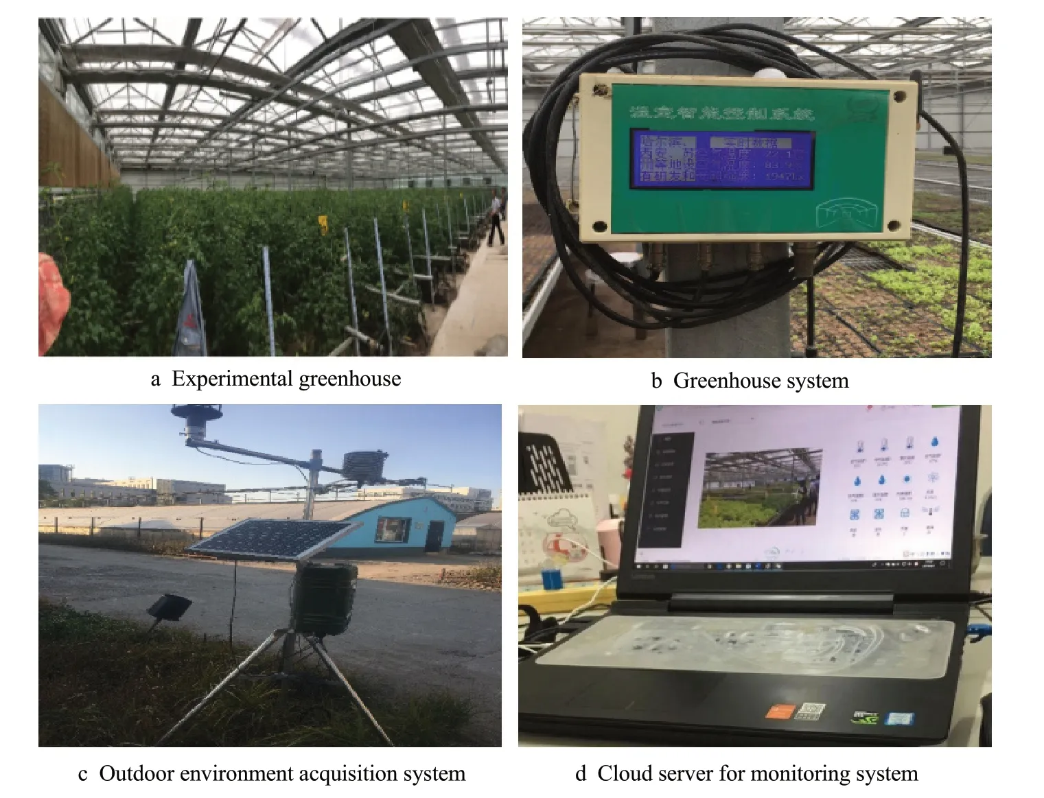
Fig. 1 Experimental greenhouse and equipment layout

Data sampling in greenhouse

The data for the environmental variables and control equipment (fans, wet curtains, sprays, sunshades and top windows) were recorded every 5 min to establish the greenhouse environmental monitoring. Each impact factor had a total of 288 data points collected every day. The time series of the original environment variables from 9: 00 a.m. on July 20 to 22: 00 p.m. on July 21 are shown in Fig. 2.

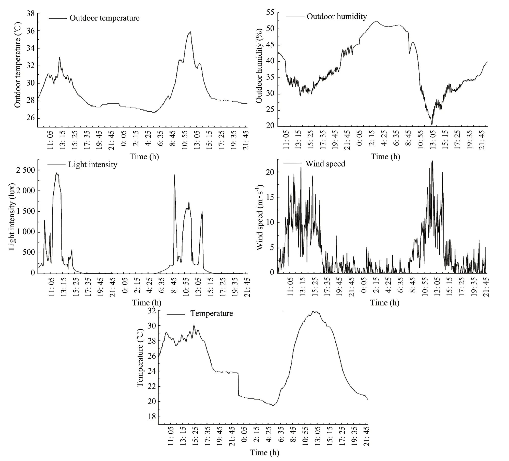
Fig. 2 Time series of original data

It could be seen from Fig. 2 that the temperature and light intensity in the greenhouse increased significantly at approximately 11: 00 a.m. and the change was relatively large. Thus, the manager should cool down the greenhouse at this time, and the corresponding control equipment should be opened until the temperature reached the optimal point for tomato growth.

The greenhouse temperature prediction model proposed in this paper was developed by employing a comparative analysis with a RBF neural network and a time series model, and energy saving comparisons of the optimization decisions of the multi-objective function were made by using NSGA-II and NSGA on this basis.

RBF neural network

RBF neural network had the advantages of high approximation accuracy, a small network scale, high computational efficiency, and no local minimum problem. Its structure consisted of three layers, namely, the input layer, the hidden layer and the output layer. The input layer was composed of signal source nodes, and it played the role of transmitting data in the functions. The neuron basis function was the most important feature of RBF, and its nodes were added through successive optimization calculations until the requirements were met. The output layer linearly weighted the information output by the hidden layer neurons to respond to the input mode. The structural design of RBF is shown in Fig. 3.

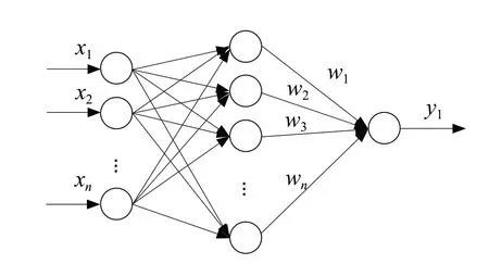
Fig. 3 Schematic diagram of RBF neural network

The radial basis function (Gaussian kernel function) in the hidden layer was expressed as the following:

Where,φj(x) was the output of thejth unit of the hidden layer,xwas the input vector,cjwas thejth Gaussian nuclear unit center andEwas an-dimensional unit vector.σjwas the variance of the Gaussian function. ||x-cjE|| was the Euclidian norm and was usually expressed as the following: The output layer was represented by a linear weighted combination of hidden layer nodes, which could be expressed as the following:

Where,hwas the number of hidden layer nodes, andwwas the weight value from thejth hidden layer node to thekth output layer node.

Time series model

The time series model ARMA (Zuoet al., 2010) could be expressed as the following:

The model was set asDetito ARMA(p,q), whereprepresented the order of the autoregressive part;φjrepresented the autoregressive coefficient, wherej=1, 2, 3, …,p;airepresented the residual sequence;qrepresented the moving average partial order; andθkrepresented the moving average coefficient, wherek=1, 2, 3, …,q.

NSGA-II multi-objective optimization algorithm

Multi-objective optimization problem

In practical problems, there were multiple optimization goals. There were often contradicting and conflicting issues between them. It was difficult to find an optimal solution that could simultaneously satisfy all the optimization goals for this problem. The mathematical expression of the multi-objective optimization problem consisting ofmdecision parameters andntarget variables (Ahnet al., 2009) was as the followings:

x=(x1,x2, …,xm) represented am-dimensional decision parameter,y=(f1(x),f2(x), …,fn(x)) represented an-dimensional objective function,gi(X)≤0 represented all the inequality constraints, andhi(X)=0 represented all the equality constraints.

NSGA-II

(1) Code generation: the greenhouse system decision parameters were binary coded and a chromosome contained all the permutations and combinations of the decision parameters. The role of the chromosomes contained in the model was to determine whether the requirements were met for each plan, and each chromosome represented a decision-making scheme.

(2) The initialization of the population and calculation of the fitness: an initial population was generated according to the coding rules of chromosomes. To calculate the fitness, the fitness function must be determined firstly. According to the decision parameter allocation scheme corresponding to the given chromosome, the objective functions were calculated as required. Fast non-dominated sorting based on the target values for all the chromosomes in the generated population was carried out. After the iterative evolution was completed, the Pareto optimal solution set with more uniformity and diversity was searched.

(3) Crowding distance and crowding comparison operator: the crowding distance referred to the smallest rectangle that contained the individual itself near a specified point in the group, but did not contain other individuals.

(4) Select operation: this operation generated the next generation of excellent individuals with good fitness based on the principle of NSGA-II and through the comparison of the fast non-dominated sorting and crowding operators using tournament selection. The tournament selection valuekwas usually equal to two.

(5) Crossover and variation: the crossover and mutation operations were carried out uniformly for chromosomes. Both the paired chromosomes and the crossover positions were randomly selected. The individuals on whom crossover was performed varied with a fixed probability.

Experimental research

To verify the accuracy of the predicted temperature of RBF model and the energy saving effect of NSGA-II optimization decision parameters, the following experimental scheme was designed.

(1) The experiment data from July 1 to July 25 were selected as the training data. RBF neural network and time series models were used to construct the greenhouse temperature model. The experiment data from 9:00 a.m. of July 26 to 11:30 a.m. of July 30 were used as the test data. The actual values in the greenhouse were compared with the predicted values of the greenhouse model.

(2) The data from 11: 30 a.m. to 2: 00 p.m. on July 30 were selected for the multi-objective optimization control. The decision parameter combination was changed every 5 min during the experiment. The combinations of RBF neural network and NSGAII and of RBF neural network and NSGA were used to optimize the decision parameters of the fans, wet curtains, sprays, sunshades and top windows. The simulation time of the experiment was 2.5 h. Then, the relationships were observed between the objective functions.

(3) Field verification was conducted according to the combination of decision parameters with the lowest temperature error and the highest energy consumption after the simulation optimization. The greenhouse environment was controlled at 11: 30 on July 31. At this moment, the temperature in the greenhouse was 31℃. According to the season, the optimal temperature of the tomatoes was 25℃, and thus the greenhouse was cooled down. The decision parameters were replaced by the NSGA-II optimized results when the temperature was 25℃. The monitoring value of the temperature sensor in the greenhouse was observed and the energy consumption value was calculated.

Multi-objective optimization of decision parameters

Greenhouse environment modeling

Since the greenhouse was a real-time, changing, complex, nonlinear and interactive microclimate system, RBF neural network used in this study could mine the potential regular characteristics of the environmental data. A nonlinear mapping relationship was established, according to the input and output relationship of the research object.

The input layer variables affected the greenhouse temperatureviadisturbance parameters and decision parameters. The disturbance parameters were the temperature outside the greenhouse, the humidity outside the greenhouse, the light intensity in the greenhouse and the wind speed outside the greenhouse.The decision parameters were divided into the controlling device switching states (fans, wet curtains, sprays, sunshades and top windows) that affected the environmental variables. Since these data units and data sizes were different, these data were normalized as the following:

In the equation,xnormalizedrepresented the result of normalizing the input layer data,xirepresented the variable input value,xrepresented the arithmetic mean,xmaxindicated the maximum value of the input,xminindicated the input minimum value and the value ofxnormalizedwas from [0, 1].

Greenhouse temperature control model

To calculate the time for the continuous operation of the control equipment, when the greenhouse tomatoes reached the adaptive growth environment parameter, the environmental control effect model for the combination of greenhouse control equipment was instituted as the following (Gu and Mao, 2001):

Where,Tt0was the temperature at timet0,Ttwas the temperature at timet,UTwas the comprehensive influence coefficient of the external climate change for the greenhouse temperature,CTjwas the correction factor when controlling the equipment state combination,niwas the amount of work for the control equipment,kiwas the control equipment switch,iwas the amount of the control equipment number,FTiwas the influence factor for controlling the state change of the equipment and the external climate with respect to the temperature in the greenhouse,Ttiwas the influence coefficient for the greenhouse temperature when the control equipment worked alone, andt-t0was the time that the continuous control equipment worked.

Greenhouse system energy consumption modeling

According to the actual situation of the greenhouse, a greenhouse energy consumption model was established (Wuet al., 2007).

Where, ∑7i=5xiPitiwas the amount of electricity consumed by the continuous control equipment, such as the fans, wet curtains and sprays; and ∑9

j=8xjQjtjrepresented the amount of electricity consumed by the non-continuous control equipment, such as the sunshades and top windows.Pirepresented the rated power of the continuous control equipment;tirepresented the continuous control equipment's actual working time for the tomatoes, which was (7)t-t0;Qjrepresented the rated power of the non-continuous control equipment operated to fully open;tjindicated the actual working time of the non-continuous control equipment for the tomatoes; andxiandxjindicated the switch status of the control equipment, where "0" meant OFF and "1" meant ON.

Optimization of greenhouse decision parameters based on NSGA-II

Based on the above model, the target was to achieve the highest temperature accuracy and the lowest energy consumption suitable for tomato growth. The multi-objective function of the greenhouse temperature error model and energy consumption models were established as the followings:

Where,f1was an error function that was constructed on the basis of RBF neural network,f2was the above greenhouse energy consumption model,simwas RBF neural network prediction function,sim(net, [x1,x2,x3,x4,x5,x6,x7,x8,x9]) was RBF neural network prediction temperature function, net was a network training model based on RBF neural network andtset was the optimum temperature for tomato growth of 25℃.

According to the experimental data collected at noon in the greenhouse, the constraints were set as the followings:

The disturbance parametersx1-x4were the temperature outside the greenhouse (℃), the humidity outside the greenhouse (%), the light intensity (lux) in the greenhouse and the wind speed (m • s-1) outside the greenhouse. The decision parametersx5-x9were the switch status of the fans, wet curtains, sprays, sunshades and top windows. The decision parameters were a random permutation combination under the constraints of the disturbance parameters and RBF neural network prediction temperature function.

Based on the above analyses, a RBF neural network and NSGA-II were used for the greenhouse multiobjective optimization control, and the specific implementation steps are shown in Fig. 4.

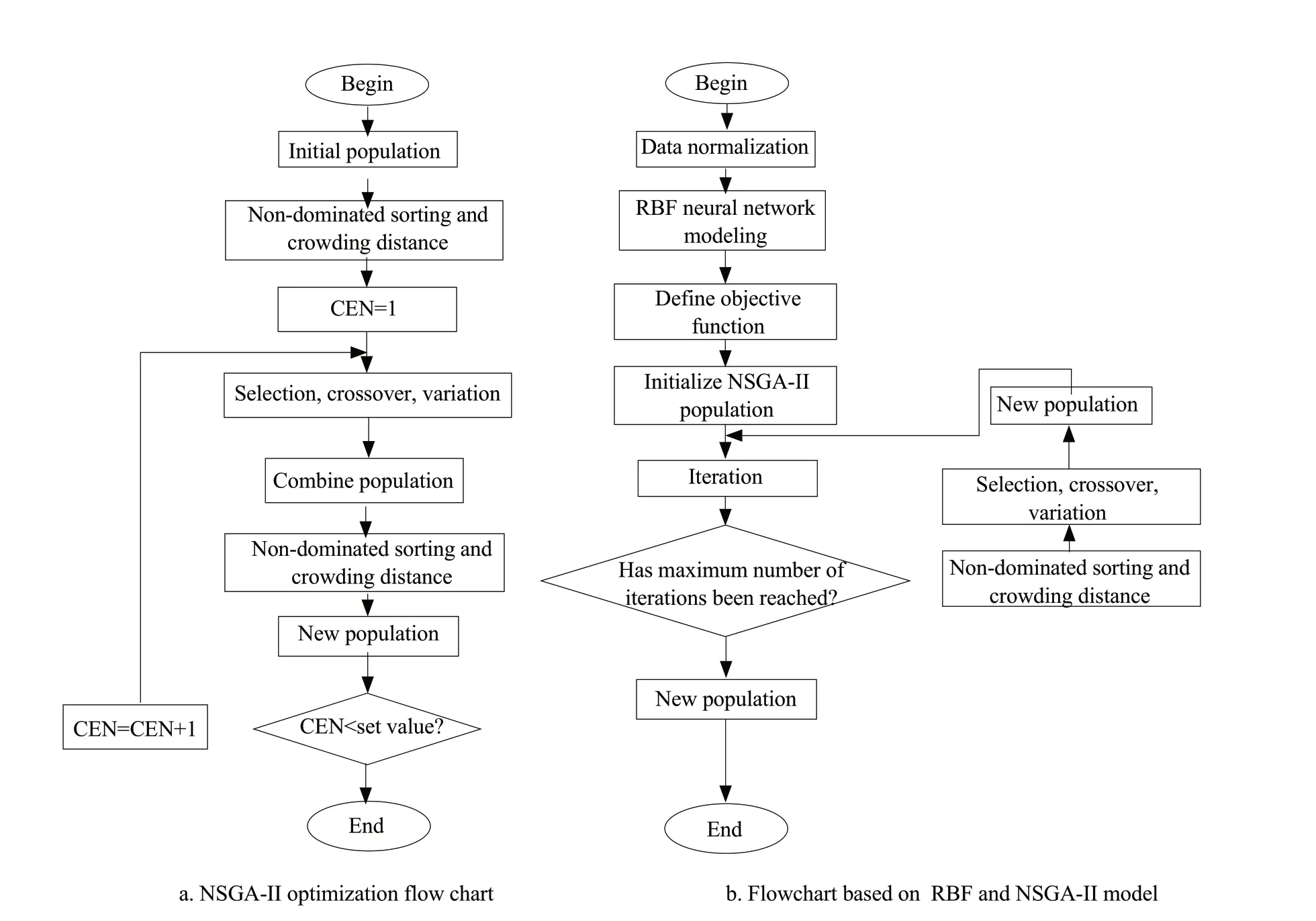
Fig. 4 NSGA-II algorithm and implementation flow of multi-objective model

Results

Prediction and simulation results

RBF neural network was used for learning and training. The input layer of RBF network of the training data included the disturbance parameters, the decision parameters and nine input nodes. The output layer was the predicted value of the greenhouse temperature and had one node. In this study, RBF adopted the feedforward neural network structure and had local approximation network characteristics. The number of hidden layer nodes was 13, the radial basis network transfer function wasnewrb(.), and the test network prediction function wassim(.). The iterative process of RBF neural network in the training process is shown in Fig. 5.

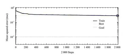
Fig. 5 RBF neural network training process

It could be seen from Fig. 5 during the parameter training process, the learning accuracy was set to 10-2and the number of iteration steps was nearly steady at 1996 steps. At this time, the best training error obtained was 0.62℃.

To verify the algorithm's performance, the prediction results of RBF and the time series models for the test data were compared with the original sequence, as shown in Fig. 6. RBF model had better prediction performance.

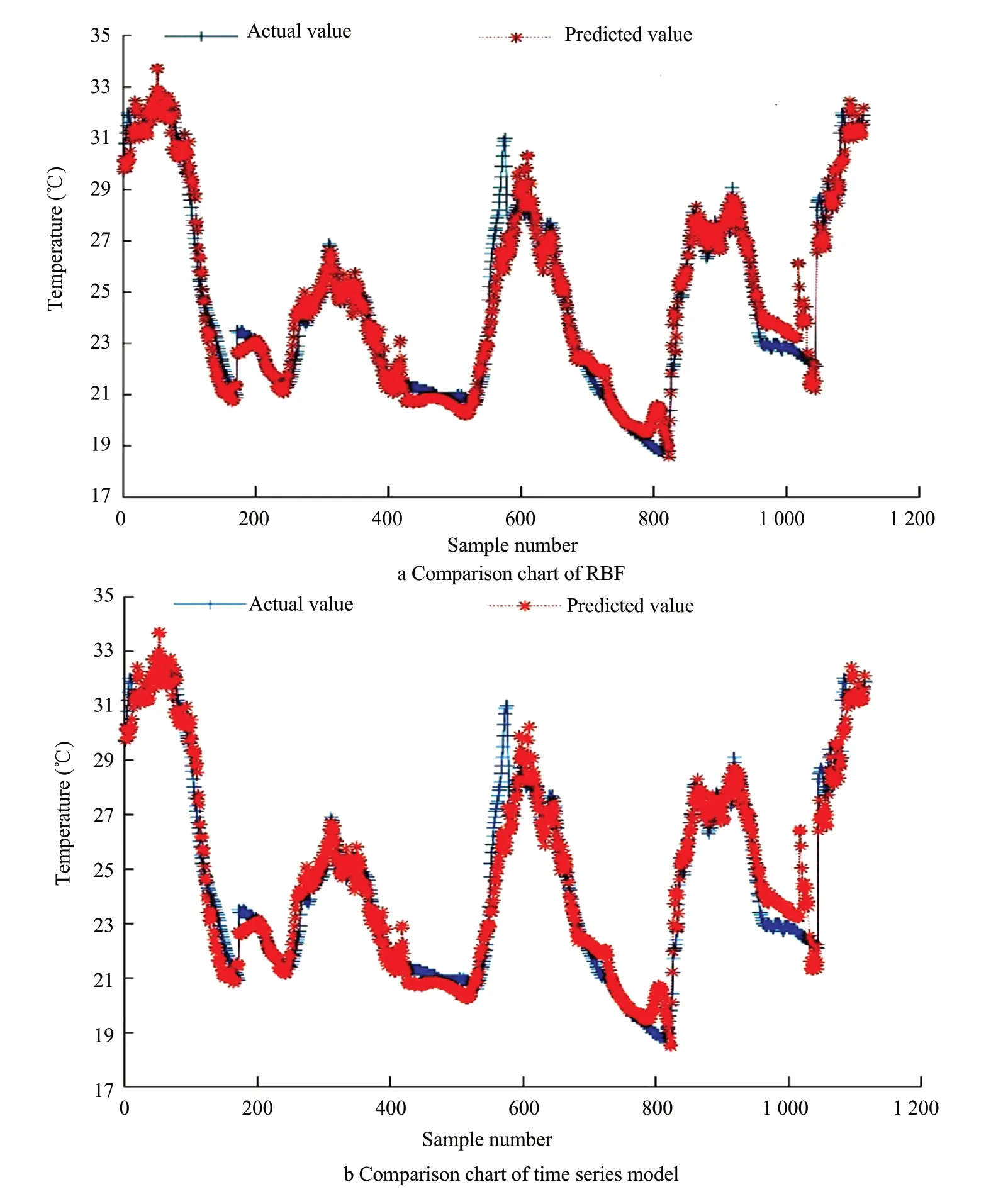
Fig. 6 Comparison of actual and predicted values of temperature of two schemes

The relationship between the predicted and actual values of the greenhouse temperature is shown in Fig. 7. The results showed that the correlation coefficientR2between the predicted results of RBF neural network and the actual value was 0.95, and the correlation between the predicted value and the actual value was higher.

To further validate the applicability of RBF prediction model to the greenhouse, the mean squared error (MSE), mean absolute percentage error (MAPE) and correlation coefficient (R2) of RBF neural network and the time series models for the test data were used as the evaluation indexes and compared, as shown in Table 1. MSE indicated the degree of dispersion of the model, the mean absolute error (MAE) reflected the actual prediction error, and the MAPE measured the prediction accuracy. The smaller the value was, the more accurate the prediction would be. The closer the correlation coefficient was to 1, the stronger the comprehensive ability of the prediction model, the higher the prediction accuracy would be.

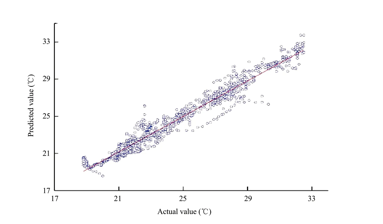
Fig. 7 Curve fitting of actual and predicted values

Table 1 Evaluating two methods of predicting temperature

As shown in Table 1, RBF neural network prediction results were more accurate than the time series model prediction results. The correlation coefficient (R2) was 0.95, MAE was 0.58℃ and MSE was 0.66℃, which reflected that the actual prediction error of RBF was lower than that of the time series model. The results indicated that the model was less discrete. The mean absolute percentage error (MAPE) of RBF model reflected the relative error of 1.49%, which was lower than that of the time series model. This showed that the predicted values were more accurate and had a strong generalization ability. Furthermore, the correlation coefficient (R2) of RBF neural network prediction results was higher than that of the time series model, which showed that RBF could more effectively simulate the greenhouse environment temperature change and meet the requirements of the subsequent multi-objective optimization decision parameters.

Multi-objective optimization results and analysis of greenhouse environment

The simulated population size was set asN=30 and the maximum number of iterations as GENmax=100, and the results almost reached a near convergence state. The number of optimization decision variables was set to 5, and the optimization objective function was 2. The simulation results are shown in Figs. 8 and 9.

Fig. 8 showed that the temperature error of the online control decreased as the energy consumption increased. The results showed that the energy consumption and temperature error were conflicting objective functions. After the algorithm was iterated 100 times, it reached the front edge of the Pareto response. Furthermore, it was found that the uniformity of the Pareto solution set optimized by NSGAII algorithm was better than that of NSGA algorithm. By taking some points optimized by NSGA-II and NSGA, points A and A' in Fig. 8 illustrated, when the temperature errorf1was 0.04℃, the corresponding energy consumption off2was 0.22 MJ and 0.38 MJ, respectively. Compared with the NSGA, the energy consumption of NSGA-II optimization system was reduced by 72%. Therefore, a more satisfactory equilibrium solution could be found from Fig. 8 and decision makers could choose the combination of decision parameters that was suitable for the growth of tomatoes to achieve the lowest energy consumption.

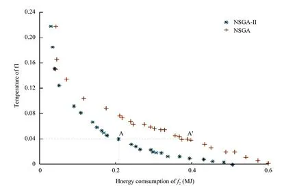
Fig. 8 Pareto solution after 100 iterations

Fig. 9 showed the temperature response of NSGA-II and NSGA to greenhouse temperature control. The 2.5 h of control were divided into 10 control steps, and the control period was 15 min. Thex-coordinate was the time point, and they-coor-dinate was the temperature value. During the simulation process, the number of simulation iterations to achieve optimal growth temperature of 25℃ was selected as the standard. Under this condition, Fig. 9 showed the temperatures at different time points with the combination of decision parameters with the lowest energy consumption, and showed the response from 31℃ to 25℃ at different time points. The temperature controlled by NSGA-II was shown to be close to a steady state at the 3rd step, while the steady temperature state of NSGA control was obviously delayed and there were fluctuations. Comparing NSGA-II and NSGA, it could be seen that the control strategy of NSGA-II achieved a better control effect.

Experiment results and analysis

According to the actual situation of greenhouse decision makers who wanted to control the temperature accuracy of the greenhouse, the experiment verified that NSGA-II simulation objective function (temperature error) was minimized and the objective function (energy consumption) was maximized. At 11: 00 a.m. on July 31, the greenhouse room temperature was 31℃. After opening the sunshades and spraying for 40 min, the average temperature in the greenhouse was 25℃. The amount of electricity consumed was 0.5 MJ. At this moment, the temperature in the greenhouse was the optimal growth temperature of tomatoes.

To further simultaneously verify the temperature and energy consumption changes in the greenhouse, the actual production greenhouse that was cooled down when the temperature was above the threshold and the one that was heated up when the temperature was below the threshold was selected for comparison. The greenhouse temperature was 30.5℃ at 10: 00 a.m. on July 24 with the wet curtains, sunshades and top windows opened. The wet curtains and top windows were opened at a temperature of 32.2℃ in the greenhouse at 12: 00 a.m. on July 25.

At 11: 00 a.m. on July 26, the temperature was 31.2℃, and the fans and sunshades in the greenhouse were opened for a total of 3 days for the comparison experiment to observe the temperature after controlling and calculating the energy consumption value. Compared with the common environmental control methods commonly used in production greenhouses, the greenhouse environmental control method based on NSGA-II had great advantages in reducing the energy consumption, and the results are shown in Fig. 10. When the temperature was controlled to 25℃, the energy consumption (0.5 MJ) under the optimization of NSGA-II algorithm on July 31 was 62.5% of the energy consumption (0.8 MJ) under the control of the production greenhouse on July 24, and the energy savings was 37.5%. By reducing the temperature in the greenhouse from 32.2℃ to 26.5℃ on July 25, the energy consumption using NSGA-II algorithm was 91% of the production greenhouse control (0.55 MJ), which meant that the energy consumption reduced by 9.1%. On July 26, the production greenhouse control temperature reduced from 31.2℃ to 25.2℃. The energy consumption (0.7 MJ) was 1.4 times that of NSGA-II, and the energy consumption was reduced by 28.5%. The above results showed that the use of NSGA-II to optimize the environmental control achieved the highest temperature accuracy, and effectively reduced the energy consumption with significant energy savings.

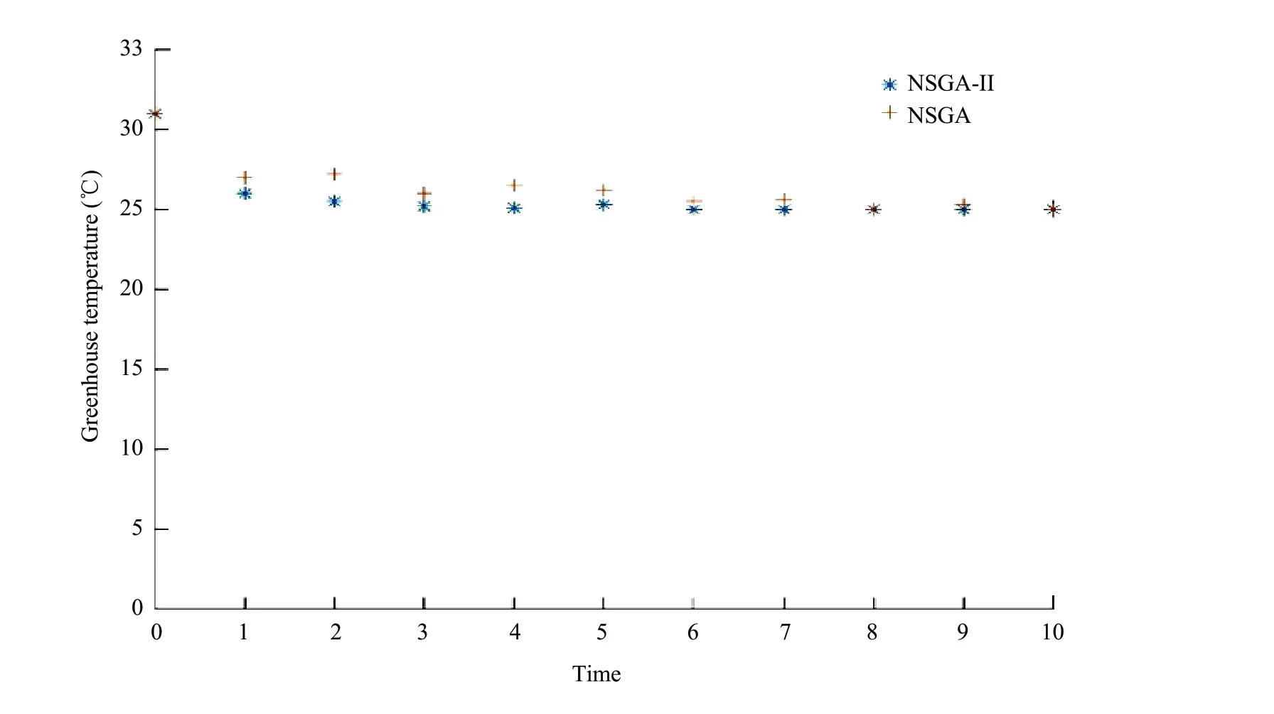
Fig. 9 Temperature response

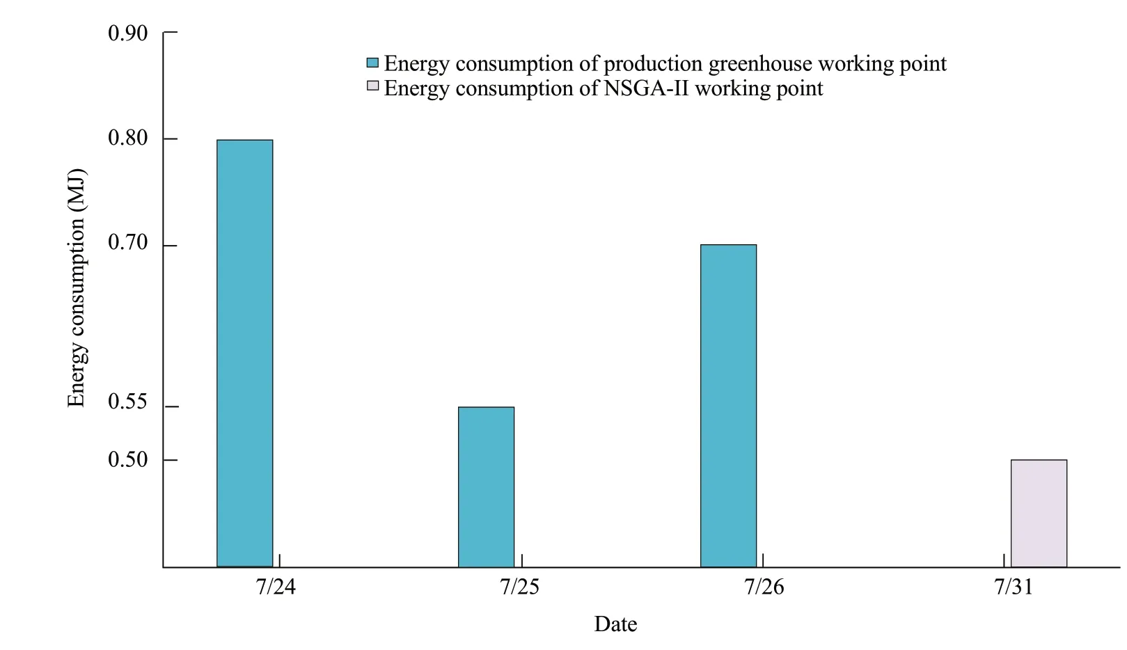
Fig. 10 Comparison of energy consumption by using two different methods for greenhouse environment control

Discussion

The greenhouse used the algorithm combined with RBF and NSGA-II for multi-objective optimization control to achieve the purpose of energy saving and consumption reduction. Using RBF neural network could further improve the prediction accuracy, the simulation results showed that RBF model was 0.58℃, 0.66℃ and 1.49% lower than the time series model, and the correlation coefficientR2was 0.95 higher than the time series model. RBF model could more effectively reflect the changes in the temperature of the greenhouse over time. There was a more uniform Pareto solution set for the objective function by using NSGA-II algorithm on this basis, the temperature adjustment had better control performance, and the advantages of short response time and small steady-state error could be achieved. Decision makers could choose the optimal plan according to the actual situation. From the test results, when the temperature accuracy reached the highest level, the energy consumption of the control equipment scheme optimized by NSGA-II was reduced by 37.5%, 9.1%, and 28.5%, respectively, compared with the production-type greenhouse control. It could be seen that adopting NSGA-II algorithm to optimize environmental control could solve the problem of greenhouse energy consumption to a certain extent.

Conclusions

RBF and NSGA-II were proposed in this paper for environmental control. RBF had a strong nonlinear fitting ability, which could advantageously map the arbitrarily complex nonlinear relationships to design a function to achieve greenhouse temperature prediction targets. On this basis, NSGA-II non-dominated sorting mechanism was used, and the crowding distance advantages were compared. The best individuals were retained in order to form Pareto optimal solutions. The research results were as the followings.

(1) Compared with the time series model by using RBF neural network, the errors between the output value of the prediction model and the target value were smaller, and it could better meet the actual situation of the greenhouse system. Compared with the decision parameters obtained by NSGA optimization, NSGA-II had a more uniform Pareto solution set for the objective functions, and the temperature had better control performance, which could achieve a short response time and small steady-state error. Therefore, decision makers could select an optimization plan based on actual conditions.

(2) When the temperature accuracy was the highest, the energy consumption of the control equipment scheme with NSGA-II optimization results were reduced by 37.5%, 9.1% and 28.5%, respectively. Compared with the production greenhouse control, the findings indicated that using NSGA-II to optimize the environmental control could solve the greenhouse energy consumption problem to some extent.

Most of the previous studies focused on maximizing crop yields, regardless of costs. This method provided a feasible solution for greenhouse multi-objective environment control that considered greenhouse temperature control and reduced energy consumption. It provided a reasonable and effective method for further obtaining the decision parameters of greenhouse environmental control. In addition, having more data resulted in a more realistic situation of the greenhouse for the neural network. Thus, constantly improving the structure of the crop model guaranteed good control results.