Vector NLS solitons interacting with a boundary*
2021-04-28ChengZhangandDajunZhang
Cheng Zhangand Da-jun Zhang
Department of Mathematics,Shanghai University,Shanghai,200444,China
Abstract We construct multi-soliton solutions of the n-component vector nonlinear Schrödinger equation on the half-line subject to two classes of integrable boundary conditions (BCs): the homogeneous Robin BCs and the mixed Neumann/Dirichlet BCs.The construction is based on the so-called dressing the boundary,which generates soliton solutions by preserving the integrable BCs at each step of the Darboux-dressing process.Under the Robin BCs,examples,including boundary-bound solitons,are explicitly derived; under the mixed Neumann/Dirichlet BCs,the boundary can act as a polarizer that tunes different components of the vector solitons.Connection of our construction to the inverse scattering transform is also provided.
Keywords: polarizer effect,solitons on the half-line,vector nonlinear Schrödinger equation,integrable boundary conditions,boundary-bound states
1.Introduction
The concept of integrable boundary conditions(BCs),mainly developed by Sklyanin [1],represents one of the most successful approaches to initial-boundary-value problems for two-dimensional integrable nonlinear partial differential equations(PDEs).The idea lies in translating the integrability of soliton equations with boundaries into certain algebraic constraints known as reflection equations,cf [1–3].As consequences,classes of soliton models,restricted on a finite interval,are integrable subject to integrable BCs [1].
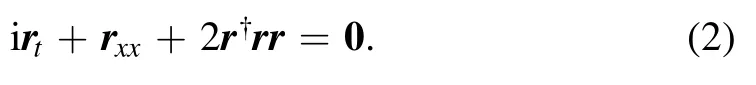
In this paper,we consider the focusing vector nonlinear Schrödinger (VNLS) equation,also known as the Manakov model [4],restricted to the half-line space domain.The equation reads

wherer=(r1,… ,r n)T,0 denotes the zero n-vector,and r†denotes the conjugate transpose of r.Each component rjis a complex field,and H is an n×n positive definite Hermitian matrix modeling interactions among the components.There is a natural U(n) -invariance of the model under the transformation r ↦T r,whereT∈U(n).Let T diagonalize H,then the VNLS equation (1),up to certain scaling,can be reduced to its standard form
The VNLS equation is a vector generalization of the(scalar) NLS equation by allowing internal degrees of freedom.Physically,it is a relevant model to describe optical solitons and collective states in low-temperature physics,cf[5,6]; mathematically,the nontrivial interactions of vector solitons are related to the notion of Yang–Baxter maps,cf[7–10].
Integrable BCs for the VNLS equation,as well as soliton solutions to the VNLS equation on the half-line,were derived in [11] by means of a nonlinear mirror-image technique [12](see also [13]) that extends the half-line space domain to the whole axis.However,there was severe difficulty constructing N-soliton solutions on the half-line as the soliton data can only be computed recursively.In practice,the computations are becoming increasingly complicated for N ≥2 (see for instance [11],conclusions).
We provide an efficient approach to deriving N-soliton solutions of the VNLS equation on the half-line.The construction is based on the so-called dressing the boundary,introduced recently by one of the authors [14,15].The essential ideas are: given integrable BCs of the VNLS equation (or any integrable PDEs),by generating soliton solutions using the Darboux-dressing transformations (DTs),we look for those DTs that preserve the integrable BCs.This gives rise to exact solutions of the underlying integrable model on the half-line,and admits a natural inverse scattering transform (IST) interpretation.The true powers of our construction consist of:(i)the N-soliton solutions can be obtained in compact forms (this was highly complicated following the mirror-image method[11,12],see the discussion provided in section 6); (ii) it does not require any extension of the space domain.This reveals that dressing the boundary represents a natural approach to solve the VNLS equation (or classes of PDEs) on the half-line equipped with integrable BCs.
Note that Fokas’ unified transform method [16,17]represents a systematic approach to treating initial-boundaryvalue problems for integrable PDEs.This method can be regarded as a generalization of the IST,cf [18–21],and was already applied to the NLS [22] and VNLS [23] equations.However,it is a difficult task to obtain exact solutions within the Fokas’ method,although asymptotic solutions at large times could be derived.
The outline and main results of the paper are as follows.First,DTs for generating soliton solutions of the VNLS equation are reviewed in section 2.Then,we recall in section 3 results on integrable BCs for the VNLS equation on the half-line[11].There are two classes of integrable BCs:the homogeneous Robin BCs and mixed Neumann/Dirichlet BCs.In section 4,we apply the approach of dressing the boundary to the VNLS equation on the half-line,which gives rise to explicit N-soliton solutions on the half-line.Our results provide a clear answer to the question of obtaining general Nsoliton solutions in the presence of a boundary [11].Moreover,we can construct stationary vector solitons subject to the Robin BCs at the boundary.These correspond to boundarybound solitons.In section 5,we provide explicit examples of vector solitons interacting with the boundary.In particular,by combining the effects of the mixed Neumann/Dirichlet BCs and the U(n) -invariance of the VNLS equation,the boundary can act as a polarizer that tunes components of solitons after interacting with the boundary.We provide connections of our construction to the IST in section 6.Possible connections of the half-line VNLS equation under integrable BCs to the Gross–Pitaevskii (GP) equation are also discussed.
2.DTs and soliton solutions
The n-component VNLS equation (2) is equivalent to the compatibility of the linear differential system
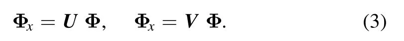
Here,U,V,known as the Lax pair,are (n+1×n+1)matrix-valued functions
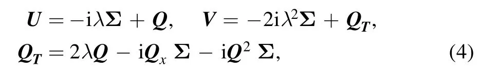
where λ is the spectral parameter,and Σ and Q are block matrices
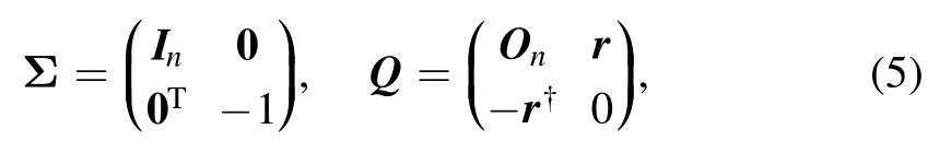
with In,Onbeing the identity and zero square matrices of size n,respectively.There is a natural gauge group acting on the Lax pair(3)
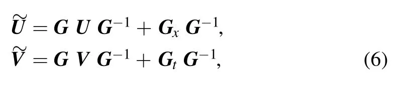
and DTs can be represented by G that preserves the forms of U,V by extracting the singular structures,cf[24–27].A onestep DT for the VNLS equation amounts to the mapwhere D[1] is called a dressing factor of degree 1
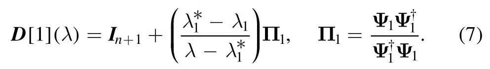
Here,Ψ1is a particular solution of the undressed Lax pair(3)associated with λ1.Having a set of N particular solutions{Ψj,λj},j=1,…,N,one can iterate the DTs and construct the dressing factor D[N] of degree N.For simplicity Ψj's are assumed to be vectors(of rank 1).In the IST formalism,D[N]plays the role of the scattering matrix: one adds a pair of complex zero/poleto the scattering system at each step of the DTs .There are two important properties of DTs:(1) the Bianchi permutativity,meaning that the order of adding Ψjis irrelevant; and (2) the action of D[N](λ) can be expressed in compact forms (usually in terms of determinant structures).
Since we are focusing on soliton solutions,the zero seed solution r=0 is imposed to the undressed Lax pair.Without loss of generality,let Ψj's be in the forms
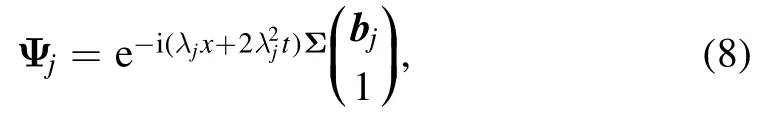
where bj's are constant complex n-vectors called norming vectors.Now,encoding the soliton data into{bj,λj},j=1,…,N,with distinct λj,the N-soliton solutions to the VNLS equation (2) are,cf [21,26]
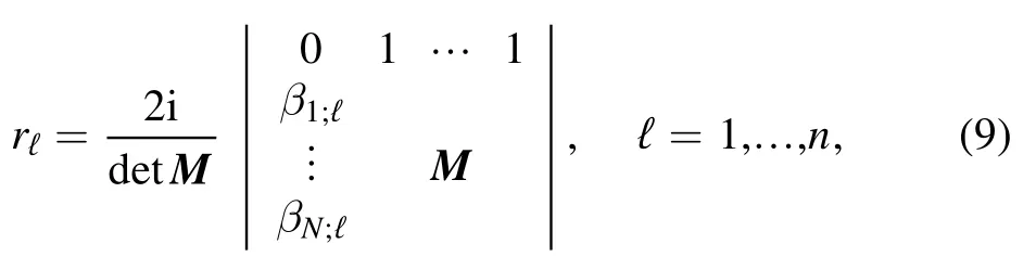
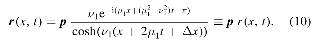
where rℓis the ℓth component of r,with βj;ℓbeing its ℓth component,and the N×N matrix M has the componentsAs an illustration,the one-soliton data {b1,λ1},withν1>0,lead to the one vector soliton solution
3.Integrable BCs for VNLS
Now we restrict the space domain of the VNLS equation to the positive semi-axis.Integrable BCs for the half-line VNLS equation were investigated in [11] (see also [28] in which only the vector Robin BCs were derived).The integrability in the presence of a boundary was translated into a constraint on the t-part of the Lax pair

Here,the boundary matrix K(λ) is assumed to be nondegenerate.As solutions of the boundary constraint(11),two classes of BCs were obtained [11]: (i) the homogeneous vector Robin BCs:

having the boundary matrix
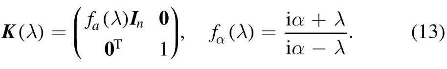
The real parameter α controls the boundary behavior: the Neumann(rx|x=0=0)and Dirichlet BCs(r|x=0=0)appear as special cases of (12) as α=0 and |α|→∞,respectively; (ii)the mixed Neumann/Dirichlet (mND) BCs:

where rℓis the ℓth component of r.Accordingly,one has the boundary matrix
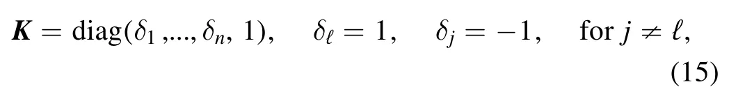
where the+/−sign of δℓcorresponds to Neumann/Dirichlet BCs.
Remark 1.The boundary constraint (11) was derived in [11]by considering the space-reverse symmetry of the VNLS equation as a Bäcklund transformation.The same constraint was also introduced in Fokas’ unified transform,known as linearizable BCs.Note that the boundary matrixKis related to a far-reaching context as it represents solutions of the classical and quantum reflection equations [1–3].
Remark 2.The integrable BCs are compatible with the U(n)-invariance of the VNLS equation.The transformationis trivial to the Robin BCs,because a collective change in the components ofrtakes place at the boundary underT.However,Tinduces a nontrivial effect under the mND BCs: since the components ofrcan interact differently with the boundary in two ways that are Neumann and Dirichlet BCs,the action ofTcan mix the two interactions and make transmissions among the different components appear.These transmission phenomena have the interpretation that the boundary acts as a‘polarizer’tuning the polarizations of the incoming solitons and,after interacting with the boundary,changes in the polarizations among the solitons take place [11].
4.Dressing the boundary
The integrable BCs for the VNLS equation on the half-line are completely determined by the t-part of the Lax pair through the boundary constraint (11).By dressing the boundary[14],we mean that in the process of DTs to generate exact solutions,the boundary constraint is preserved at each step of the DTs.By construction,this leads to exact solutions of the VNLS equation subject to the integrable BCs.In practice this requires one to find appropriate particular solutions in DTs.
Lemma 1.[Dressing the boundary] LetU,Vbe the undressed Lax pair.Assume thatVsatisfies the boundary constraint (11),and that the Lax pair admits a pair of particular solutionsassociated withrespectively (assumeλjis not pure imaginary),such that

whereK(λ)is the boundary matrix; then the boundary constraint (11) is preserved after dressingVusing Ψj,
The proof is closely related to the structure of dressing factors.Similar statements can be found in[14]for the scalar case.To obtain exact solutions on the half-line,it remains to find the paired particular solutions Ψj,satisfying (16).
Proposition 1.[N-soliton solutions on the half-line] Let{bj,λj} andj=1,…,N,be two sets of N-soliton data.Assume thatis not pure imaginary) andwithB(λ)=fα(λ)In(fα(λ)defined in (13)),then the so-constructed solutions restricted tox≥ 0 correspond to N-soliton solutions on the half-line subject to the Robin BCs(12);ifB= −diag (δ1,...,δn),δℓ= 1,δj= −1,forj≠ℓ,then the solutions restricted tox≥ 0 satisfy the mND BCs (14).
The proof is a direct consequence of lemma 1 by taking into account the forms of the particular solutions(8).Dressing the Lax pair using the N-paired soliton data {bj,λj} andgives rise to 2N-soliton solutions on the whole-line,and the requirements thatcreate solitons with opposite velocities.By restricting the space domain to the positive semi-axis,the BCs appear as interactions of solitons with opposite velocities at x=0,then one obtains N-soliton solutions on the half-line.Although this whole-line picture helps to interpret interactions of solitons as BCs,the derivation of soliton solutions on the half-line can be restricted to x ≥0.This is in contrast to the nonlinear mirror-image technique[11,12],where an extended potential to the wholeline is required.
Note that in the above construction,pure imaginary λj's,corresponding to stationary solitons are excluded.By dressing the boundary,we can also construct stationary solitons satisfying the Robin BCs.These are boundary-bound solitons on the half-line.
Proposition 2.[Boundary-bound solitons] Letβbe any realn-vector such that∣β∣= 1,and,j= 1,… ,Nbe a set ofN-soliton data.Assume thatλj’s are pure imaginary numbers and distinct,and for given α,satisfyfα(λj)<0(fα(λ)defined in (13)).Moreover,assume the following forms of the norming constantsthen the so-constructed solutions restricted tox≥ 0 correspond toN-stationary solitons on the half-line subject to the Robin BCs (12).
The requirement that β is a real vector with |β|=1 can be easily obtained by taking any real vectordivided by its normalAgain,the restriction on the soliton data follows the idea of dressing the boundary: the boundary constraint (11) is preserved at each step of the DTs.In computing the boundary-bound solitons,the expressions for the norming constants are different for the odd and even soliton numbers.One also excludes the situation where the stationary solitons are subject to the Dirichlet BCs by assuming fα(λj)<0.Note that for the scalar NLS case,the boundary-bound states were investigated in[14,29].One can put the stationary and moving solitons together by combining the associated soliton data.Due to the Bianchi permutativity of DTs,the order of adding the soliton data is irrelevant.
5.Examples of VNLS soliton interacting with a boundary
It is straightforward to apply Prop.1 and 2 to obtain soliton solutions of the VNLS equation on the half-line.Fix n=2;three examples under the Robin BCs are shown in figures 1–3.The left and right figures represent,respectively,the norms of the 1st and 2nd components of the solutions.
As for the mND BCs,fix n=2,and let the transformation matrixT∈SU(2) (following remark 2) parameterized by three parameters ω,θ,ξ be in the form
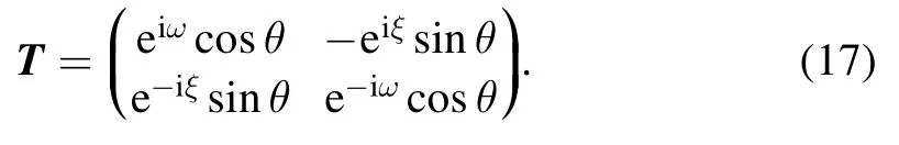
Clearly,r↦Trinduces a mixture of components of r at the boundary.In the computations of the half-line soliton solution,this amounts to B ↦TBT−1for B defined in Prop.1.Examples of two solitons interacting with an mND boundary are shown below.Having B=diag(1,−1) gives rise to solitons with the 1st component subject to Neumann BCs and 2nd to Dirichlet BCs(see figure 4);under the action of T,for certain choices of the parameters,one can make one component of the outgoing solitons vanishingly small1The complete analysis,requiring some asymptotic estimations of the solutions as t →±∞,is omitted here.Detailed analysis can be found,for instance,in [10].(see figure 5).In other words,the boundary polarizer switches off the 1st component after solitons interact with the boundary.
6.Discussion
The approach of dressing the boundary is successfully applied to the VNLS equation on the half-line.Although our construction is rather algebraic,it admits a perfect IST interpretation.Since the integrable BCs are only governed by the t-part of the Lax pair through the boundary constraint (11),the soliton data on the half-line can be derived by performing the IST using the t-part of the Lax pair on the boundary.Precisely,this amounts to the direct scattering analysis of

where QTis defined in (4).Let Φ±be the fundamental solutions (3) at x=0
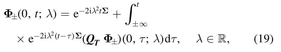
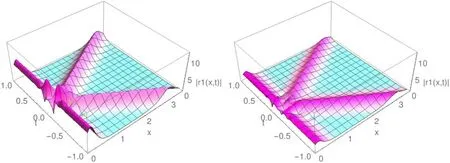
Figure 2.One soliton interacts with a boundary-bound soliton subject to the Robin BCs (α=2).The moving soliton data are: b1} andwith μ1=1.4,ν1=4,=(3 ,2) ;the static soliton data are:
Figure 3.Three stationary solitons interfere with themselves at the boundary subject to the Robin BCs (α=2).Here,

Figure 4.Two solitons interact with the mixed Neumann(1st component)and Dirichlet(2nd component)BCs with B=−diag(1,−1).The soliton data areand j=1,2 with μ1=1,ν1=2,=(4 ,4),μ2=2,ν2=1.5
they are connected by the scattering system Φ+(λ)=S(λ)Φ−(λ),where S(k) is the scattering matrix.The domain of analyticity of the components of S(k) can be split into the four quadrants of the complex plane.The boundary constraint (11) yields
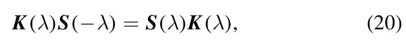
which governs the soliton data at the boundary x=0.It is easy to see that paired singularities {λj,−λj} appear (see figure 6),and the relations between the paired norming constants can also be accordingly extracted.These are the requirements listed in Prop.1.Then,making the soliton data evolve in x for x >0 gives rise to N-soliton solutions on the half-line.
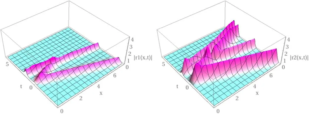
Figure 5.Polarizer effect:the boundary tunes the polarizations,and the 1st component becomes vanishingly small after interacting with the boundary.Here,the parameters in T (17) are fixed as ω=0,θ=0,ξ=50.66.
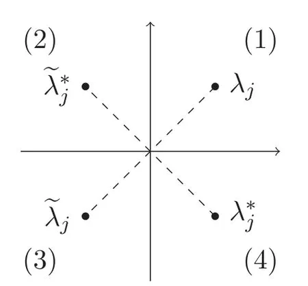
Figure 6.Pairing of soliton data in the spectral plane
Note that the relation (20) is in sharp contrast to the formulae (3.43) and (3.46) in [11],which are the governing relations of the soliton data following the nonlinear mirrorimage approach.In [11],the singularities are paired asand the paired norming constants,that are nonlinearly coupled,can be only be computed recursively.This makes the computation of N-soliton solutions on the half-line highly complicated.However,the relation (20) only involves linear relations between the paired norming constantsin Prop.1).Therefore,the half-line N-soliton solutions can be easily derived.
As pointed out by Fokas,the scalar NLS equation on the half-line under the Robin BCs can even model solutions to the GP equation on the whole-line with a Dirac-function potential at the origin,cf [30],introduction.Similarly,the VNLS equation on the half-line under the integrable BCs can also describe certain special cases of the vector GP equation.Fix the number of components n=2,and one has the vector GP equation
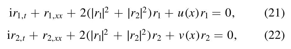
where u(x),v(x) are the potentials. Let u(x)=v(x)=−4αδ0(x),and let r1,r2be even in x.Then,after integration,the Dirac function δ0(x) introduces a jump in the derivatives
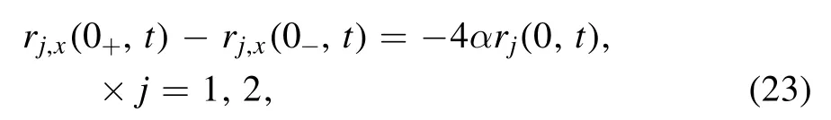
which corresponds to the half-line VNLS equation under the vector Robin BCs (12).Again,let u(x)=0,v(x)=δ0(x),and let r1be even and r2be odd in x.This corresponds to the halfline VNLS equation under the mND BCs(14),with r1and r2satisfying,respectively,the Neumann and Dirichlet BCs.
ORCID iDs
杂志排行

Communications in Theoretical Physics的其它文章
- Charged torus-like black holes as heat engines
- Pure annihilation decays of and in the PQCD approach
- Exploring the latest Pantheon SN Ia dataset by using three kinds of statistics techniques
- Hawking temperature of Kerr anti-de-Sitter black hole affected by Lorentz symmetry violating*
- The vacancy defects and oxygen atoms occupation effects on mechanical and electronic properties of Mo5Si3 silicides
- Deposition pattern of drying droplets