Stereo Matching Method Based on Space-Aware Network Model
2021-04-27JilongBianandJinfengLi
Jilong Bianand Jinfeng Li
1College of Information&Computer Engineering,Northeast Forestry University,Harbin,150040,China
2College of Computer&Information Technology,Mudanjiang Normal University,Mudanjiang,157011,China
ABSTRACT The stereo matching method based on a space-aware network is proposed,which divides the network into three sections:Basic layer,scale layer,and decision layer.This division is beneficial to integrate residue network and dense network into the space-aware network model.The vertical splitting method for computing matching cost by using the space-aware network is proposed for solving the limitation of GPU RAM.Moreover,a hybrid loss is brought forward to boost the performance of the proposed deep network.In the proposed stereo matching method,the space-aware network is used to calculate the matching cost and then cross-based cost aggregation and semi-global matching are employed to compute a disparity map.Finally,a disparity-post processing method is utilized such as subpixel interpolation,median filter,and bilateral filter.The experimental results show this method has a good performance on running time and accuracy,with a percentage of erroneous pixels of 1.23%on KITTI 2012 and 1.94%on KITTI 2015.
KEYWORDS Deep learning;stereo matching;space-aware network;hybrid loss
1 Introduction
Stereo matching is an important research topic in the field of computer vision.It is widely used in three-dimensional reconstruction [1],autonomous navigation [2,3],and augmented reality [4].In the pipeline of stereo matching,an input of stereo matching consists of two epipolar rectified images taken from different points of view,one of which serves as a reference image and the other as a matching image.For each pixel(x,y)in the reference image,stereo matching identifies a pixel(x−d,y)in the matching image,corresponding to the same points in the scene,wheredis the disparity of the pixel(x,y).According to the principle of triangulation,the depth of the pixel(x,y)can be calculated aswherefis focal length andBis baseline length.
Stereo matching process is divided into four steps:Cost calculation,cost aggregation,disparity calculation,and disparity refinement [5].Cost calculation is the first step in stereo matching process,and its quality largely affects the accuracy of stereo matching.For the past few years,deep learning has made great progress and is widely applied in intelligent traffic [6–9],network security [10–14],privacy-protecting [15–18],and natural language processing [19–21].Recently,deep learning has also been applied to stereo matching to calculate matching cost because of its powerful feature representation ability.It can improve the robustness of matching cost to radiation difference and geometric distortion and enhance matching accuracy.Lecun et al.[22,23] first employs Siamese network structure [24] to calculate matching cost,the matching cost is aggregated by the cross-based cost aggregation method,a disparity map is produced by the semi-global matching method [25],and finally,a disparity map is refined using some disparity post-processing methods.Subsequently,Zagoruyko et al.[26] extends the Siamese network structure and proposes three network structures,which are applied to stereo matching to calculate matching cost.Chen et al.[27] put forward a deep embedding model,which was like the central-surrounding twostream network [26].Luo et al.[28] propose an efficient deep learning model,which takes image patches of different sizes as input of left and right branch networks.The right image patch is larger than the left image patch in size and contains all disparities.In stereo matching,deep learning is used to calculate matching cost,which has achieved good matching results.This kind of method associates the depth of a network model with the size of training patches and the network depth depends on the size of a training image patch.As a result,it is impossible to increase the network depth to achieve high matching accuracy without changing the size of training image patches,which makes this method unable to effectively use excellent deep network structures such as residual network [29] and dense network [30].
To increase the depth of the network and improve matching accuracy,we propose a stereo matching method based on the space-aware network.Firstly,matching cost is calculated by using a deep network,then the matching cost is aggregated by cross-based cost aggregation method,and a disparity map is computed by the semi-global method.Finally,the disparity map is further refined by some disparity post-processing methods.The main contributions of this paper are as follows:Firstly,we propose a space-aware network model,which can have the ability to integrate many popular network models.Secondly,a hybrid loss function is designed to enhance the network performance.Finally,a vertical splitting method is proposed to calculate feature maps for a whole image to reduce the consumption of GPU memory.
2 Space-Aware Network Model
2.1 Basic Model
Deep learning is applied to calculation of matching cost and can produce good matching results [23].The deep network is called Siamese network,which consists of two parts:Feature layer and decision layer,and its network structure is shown in Fig.1.The feature layer is composed of two branches with the same structure and weight,which receive an image patch,respectively.The two image patches are fed into convolution layers,ReLU layers,and max-pooling layers.When they pass through a convolution layer,their size will be decreased.Finally,each branch obtains a one-dimensional feature vector,and these two feature vectors are concatenated and fed into a decision layer.The decision layer consists of a linear fully connected layer followed by a ReLU layer and outputs a scalar value,which is a probability value and denotes whether left and right image patches are similar.Fig.1 shows a deep network including 4 convolution layers with a convolution kernel of size 3×3 and the depth of this network model determines its input of size 9×9.In other words,the size of training image patches is subject to the count of convolution layers.When the kernel size is fixed,the more convolution layers are,the larger the image patch size is.This characteristic of the network model limits its depth and the application of ResNet [29] and DenseNet [30].If the network depth is deepened,it will inevitably increase the size of training image patches,which will cause over-fitting.
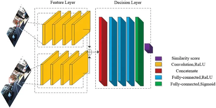
Figure 1:Deep network for stereo matching
2.2 Residual Model
He et al.[29] proposed a residual network model,which has been applied to image classification and achieved very good results.Up to now,it is still a popular network model and there are many variants.The basic idea of this model is to add an Identity Shortcut Connection to the network model,which skips several convolution layers at one time.A residual block structure is shown in Fig.2.A residual block can be expressed asH(X)=F(X)+X and is composed of two parts,one part of which is called residualF(X)and the other part is identity mapping X.In general,a residual block consists of two or three convolution layers,and these residual blocks comprise a residual network.
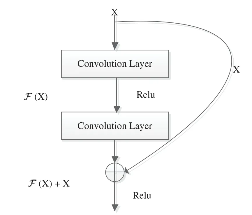
Figure 2:Residual block
The idea of residual connection is extended to propose a dense connection network [30].As shown in Fig.3,each convolution layer in a dense block has an Identity Shortcut Connection connecting to the convolution layers coming before it.The input of each convolution layer is made of the concatenation of feature maps of all convolution layers coming behind it along feature dimension.A layer in a dense block can be denoted asXℓ=Hℓ([X0,X1,...,Xℓ−1]),whereXℓis the output of the layerℓand [X0,X1,...,Xℓ−1] represents the concatenation of feature maps,Hℓdenotes a composite function of three consecutive operations:Batch normalization (BN),followed by a rectified linear unit (ReLU) and a 3×3 convolution.A DenseNet consists of these dense blocks followed by transition layers.A transition layer is mainly composed of normalization layers,1×1 convolution layers,and pooling layers.
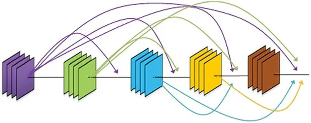
Figure 3:Dense block
2.3 Space-Aware Network Model
For each pixelpin a reference image,stereo matching first calculates matching costc(p,d),which forms a cost volume.Then,a series of steps such as cost aggregation,disparity calculation and disparity refinement are performed,and finally,a disparity map is obtained.In general,absolute values of gray difference,normalized cross-correlation function and so on are used to calculate matching cost.This paper will present a method for computing matching cost by using deep learning.At present,the size of a training image patch depends on the number of convolution layers in the deep learning-based methods for computing matching cost.If the number of convolution layers is increased to obtain more accurate matching cost,the size of training image patches will be large,which results in over-fitting and reduces matching accuracy.
To solve this problem and use a more advanced network model to calculate the stereo matching cost,we propose a space-aware network model.The main characteristic of this model is that the feature layer is divided into two parts:Basic layer and scaling layer.The main purpose of the basic layer is to extract features,which can use advanced network models such as residual network and dense network.Fig.4 shows the overall structure of the space-aware network model.The input of the basic layer is a pair of the image patchesPatchL(p)andPatchR(p−d)of size 9×9,and the output of the basic layer is the feature maps of size 9×9.In the basic layer,the size of feature maps is the same as the size of input.However,the main purpose of the scaling layer is to reduce the spatial size of feature map to 1×1.Our proposed scaling layer consists of only one convolution layer,whose size is the size of image patches.We do not choose max-pooling layer or average pooling layer.This is because the scaling convolution layer is like cost aggregation based on filter and thus can gather more space information to learn more discriminative features.For instance,when the training image patches of size 9×9 are taken as input of the network model,the filter kernel size of the convolution layer in the scaling layer is selected as 9×9.When the training image patches of size 9×9 are fed into the basic layer,the feature maps of size 9×9 are produced.Subsequently,these feature maps are fed into the scaling layer and the scaling layer outputs the feature maps of size 1×1.Finally,the feature maps of left and right image patches are concatenated to form a one-dimensional vector,which is taken as input to a decision layer,whose output is a probability,denoting the similarity between the left and right image patches.
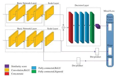
Figure 4:Space-aware network
3 Hybrid Loss
Because the proposed network model consists of three parts:Basic layer,scaling layer and decision layer,we combine the outputs of these three parts to define a hybrid loss function.The outputs of two branches of the basic layer are flattened to a one-dimensional vector,and then the cosine similarity is calculated by using an inner product layer:

whereuLanduRdenote the output of the left and right branches of the basic layer.The output of the left and right branches in the scaling layer is a one-dimensional vector,so we do not need to flatten the scaling layer output and can directly utilize the cosine similarity.Because ReLU is used as an activation function,the output of the network is greater than 0,and the output range of the inner product layer is [0,1].For these two outputs,Hinge loss is used:wheres1+ands1−denote the output of the basic network layer for positive and negative samples,s2+ands2−represent the output of the scaling layer for positive and negative samples,mis a constant and is set to 0.2 during training.For output of the decision layer,mutual entropy loss is used:


wherev+andv−are outputs of the decision layer for positive and negative samples.Finally,the total loss is:

whereθis a constant and is set to 0.3.
4 Vertical Splitting Method
During training,the proposed deep network produces three outputs:One output of the decision layer and two outputs of the inner product layer,but only the output of the decision layer is used as matching cost to compute disparities:

wherePatchL(·)andPatchR(·)denotes left and right image patches respectively,andnetwork(·)denotes the output of the decision layer.To calculate an initial cost volume by using the spaceaware network,it is necessary to take as input to the network the left and right image patches for every pixel in a reference image and the corresponding pixel in a matching image at all possible disparities.The advantage of this method is that it can reduce the consumption of GPU memory,but greatly increase the running time.An alternative method [23] uses a whole image as input to calculate matching cost.This method only calculates a feature map for left and right images one time,so it can greatly decrease running time and improve efficiency,but this method requires more GPU memory.
Therefore,we propose a vertical splitting method to reduce the consumption of GPU memory.The main idea of this method is to divide left and right images into several patches vertically:

wherepydenotes vertical coordinate ofpandKdenotes patch height.Then,an initial cost volume is produced for each pair of vertical patches using the space-aware network:

whereIiL(·)andIiR(·)denotesith patch of left and right images,respectively.Finally,these subcost volumesCiCNN(p,d)are concatenated vertically to form a complete cost volumeCCNN(p,d).
5 Disparity Calculation
The output of the space-aware network is an initial 3D cost volume.Cost aggregation,disparity calculation,and disparity postprocessing are used to obtain a more accurate disparity map.Firstly,cross-based cost aggregation is employed,and secondly,semi-global matching is adopted.Finally,a series of disparity post-processing methods are utilized,such as left-right consistency check,sub-pixel enhancement,median filtering,and bilateral filtering.
5.1 Cross-Based Cost Aggregation

The cross-based cost aggregation method [31] firstly constructs a cross arm for each pixel,then uses cross arms to define a supporting area for each pixel.A left-arm of the pixelpcan be defined as:whereI(·)represents a gray value,αandβis a predefined gray threshold and a predefined distance threshold,respectively.Eq.(8) shows that pixel pointpis taken as a starting point,and continuously extends to the left under the constraint of the predefined gray threshold and predefined distance threshold.right(p),top(p)andbottom(p)of the pixelpare constructed in the same way.After these arms are defined,the supporting areasupport(p)can be defined as:

Then,cost aggregation is carried out on the supporting areasupport(p):

whereCCNN(·,·)denotes an initial matching cost.
5.2 Semi-Global Matching
Disparity calculation is usually classified into a local optimization method and a global optimization method.Global optimization methods generally obtain a high accuracy map,including dynamic programming,belief propagation,and graph-cut optimization.A global optimization method transforms the stereo matching problem into an energy function minimization problem:

whereDdenotes a disparity map,N(p)the neighborhood of pixelp,P1andP2the constant penalty,Dqthe disparity of pointq.The semi-global method [25] approximately solves the energy function by dynamic programming in multiple directions:

whererdenotes direction andCr(p,d)is a cost volume in directionr.The final matching cost is the sum of matching costs in all directions:

Then,disparities are calculated by the “winner-takes-all” method:

5.3 Disparity Post Processing
To improve the accuracy of stereo matching,we use disparity post-processing methods such as left-right consistency check,sub-pixel enhancement,median filtering,and bilateral filtering.There are inevitably some erroneous disparities in a disparity map,which may be caused by non-textured areas and occlusion.These erroneous disparities can be detected by left-right consistency check of left and right disparity maps,and each pixel can be marked by the following rules:

whereDL(p)is a left disparity map andDR(p)is a right disparity map.Background disparities are used to fill occlusion,and correct disparities in the neighborhood are used to replace erroneous matches.
Sub-pixel refinement can further improve matching accuracy.We use a sub-pixel refinement method based on quadratic curve fitting in the cost domain,which uses optimal matching cost and its left and right immediate matching costs to fit a quadratic curve to obtain a sub-pixellevel disparity:

whereC−=CSGM(p,d−1),C+=CSGM(p,d+1),C=CSGM(p,d).
The final step of stereo matching uses a 5×5 median filter and a bilateral filter:

whereg(·)is Gaussian function,denotes a normalized constant,andγis a predefined threshold.
6 Experimental Analysis
We use LUA and Torch7 to implement the proposed stereo matching method based on a deep space-aware network and the network is trained on GeForce GTX1080Ti GPU.The experimental parameters are set asα=4,β=0.00442,P1=1,P2=32,γ=5.The experimental data sets are KITTI 2012 and KITTI 2015.KITTI 2012 stereo dataset contains 194 training images and 195 test images,while KITTI 2015 stereo dataset contains 200 training images and 200 test images.Training data set is generated according to [6,17].The training data set is composed of positive and negative samples.Positive samples are defined as matching image patches,while negative samples are defined as unmatched image patches.The number of positive samples is the same as the number of negative samples,which can prevent it from loss of accuracy caused by imbalanced samples.
6.1 Training Strategy
The choice of training strategy is very important for deep learning,and a good training strategy can accelerate convergence and improve accuracy.In our experiment,the SGD optimizer algorithm is adopted,and its momentum is set to 0.9.The learning rate adjustment method is OneCycleLR with a cosine annealing strategy and the initial learning rate is set to 0.003.Its learning rate curve is shown in Fig.5.The space-aware network is trained for 14 epochs.
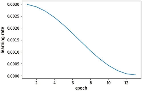
Figure 5:Learning rate curve
6.2 Classification Accuracy Analysis
The computation of matching cost with deep learning is a binary classification problem.The higher the classification accuracy is,the more accurate the matching cost is,and the higher the matching accuracy is.In this experiment,80% of training data is used as training data and 20% as validation data to analyze the classification accuracy of the proposed network model.The comparison of classification accuracy is shown in Fig.6a,which indicates that the validation accuracy increases steadily with the increase of training epochs,and our classification accuracy is 98.40%.With the increase of epochs,the classification accuracy of [22] shows a slight fluctuation and its classification accuracy is 94.25%.We also compare training loss and validation loss.The comparison of training loss is shown in Fig.6b,which indicates that our proposed method obtains lower training loss and better convergence effect.Fig.6c shows validation loss.With the increase of epochs,the validation loss of our proposed method gradually decreases,and our validation loss is lower than [22],which shows that our network model is better than [22].
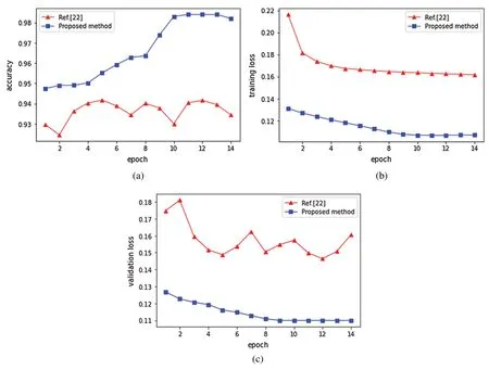
Figure 6:Classification accuracy and loss for the proposed method and Ref.[22].(a) Classification accuracy (b) Training loss (c) Validation loss
6.3 Matching Accuracy Analysis
In this paper,we implement two space-aware network models.In the first network called SADenseNet,DenseNet with 20 DenseNet blocks is selected as the feature layer,the scale layer consists of a convolutional layer with the filter kernel of size 11×11,and four fully connected layers are included in the decision layer.We train SADenseNet network on the KITTI2012 data set and the KITTI2015 data set,respectively.Then 40 stereo image pairs are extracted from every data set to calculate the average number of bad pixels of 3 pixels.The experimental results are shown in Tabs.1 and 2.The second network is called SAResNet.In this network,the basic layer is composed of the residual network of 18 residual blocks,and the scaling layer is one convolution layer of size 11×11,and the decision layer consists of four fully connected layers.The experimental results are also shown in Tab.1 and Tab.2.Disparity maps for the two proposed networks are shown in Fig.7,in which the first row is left image and ground truth;the second row is the calculated disparity map and the error map for SAResNet,in which green denotes correct disparities and red denotes erroneous disparities,and whose error percentage of 3 pixels is 0.16%;The third row shows the calculated disparity map and the error map for SADenseNet,and whose error percentage of 3 pixels is 0.46%.It can be observed from the disparity map that the error of the blue rectangle in the disparity map calculated by the SAResNet network has been improved obviously.
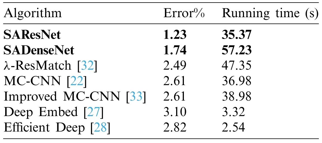
Table 1:Comparison result for 2012 dataset

Table 2:Comparison result for 2015 dataset
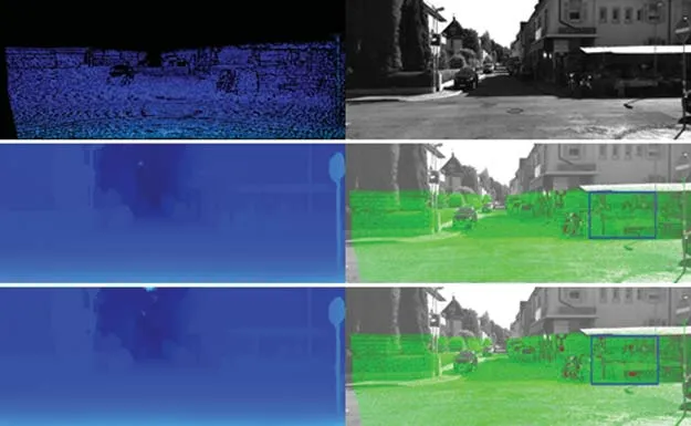
Figure 7:Comparison for disparities map of two proposed deep network
6.4 Comparision of Experimental Results
In this section,we first use the KITTI2012 dataset to test the performance of our proposed stereo matching method based on a space-aware network model and compare it with other methods.We randomly select 40 stereo pairs and compute the average error percentage of 3 pixels.The comparison results are shown in Tab.1.Our proposed method gives a good performance,whose average error percentage is 1.23%.Fig.8 shows the calculated disparity maps for four methods with low error percentage.Fig.8a shows the left and right images and the ground truth,and Fig.8b shows the calculated disparity and the error map for SAResNet,with an error percentage of 0.65%;Fig.8c for SADenseNet,with an error percentage of 1.2%;Fig.8d for [32],with an error percentage of 4.97%;Fig.8e for [22],with an error percentage of 5.90%.From these error maps,it can be observed that our method can obviously reduce the erroneous pixels in the blue rectangle.
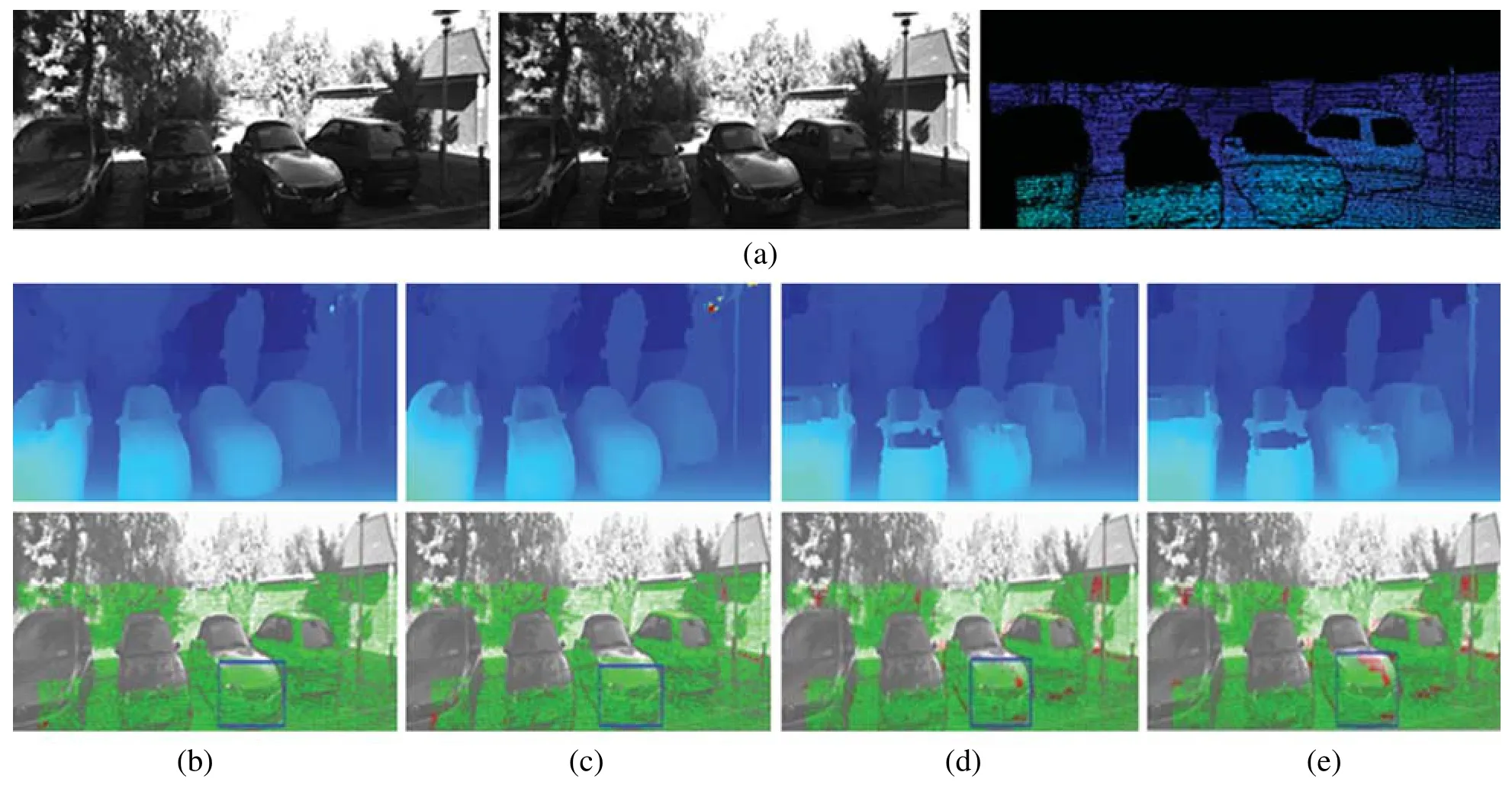
Figure 8:Results of disparity estimation for KITTI 2012.(a) The left and right images and the groud truth (b) SAResNet (c) SADenseNet (d) [32] (e) [22]
In this section,we use the KITTI2015 dataset to test the performance of our space-aware network and compare it with other methods by using the same metric as the KITTI2012 dataset.The comparison results are shown in Tab.2.Fig.9 shows the calculated disparity maps for four methods with low error percentage.Fig.9a shows the left and right images and the ground truth,and Fig.9b shows the calculated disparity map and the error map for SAResNet with the 3-pixel error percentage of 0.64%;Fig.9c for SADenseNet with the 3-pixel error percentage of 1.30%;Fig.9d for [32] with the 3-pixel error percentage of 2.80%;Fig.9e for [22] with the 3-pixel error percentage of 2.90%.These experimental results show that our proposed method can give a more accurate disparity.The blue rectangles in these error maps show that the erroneous pixels marked by red are less than other methods.
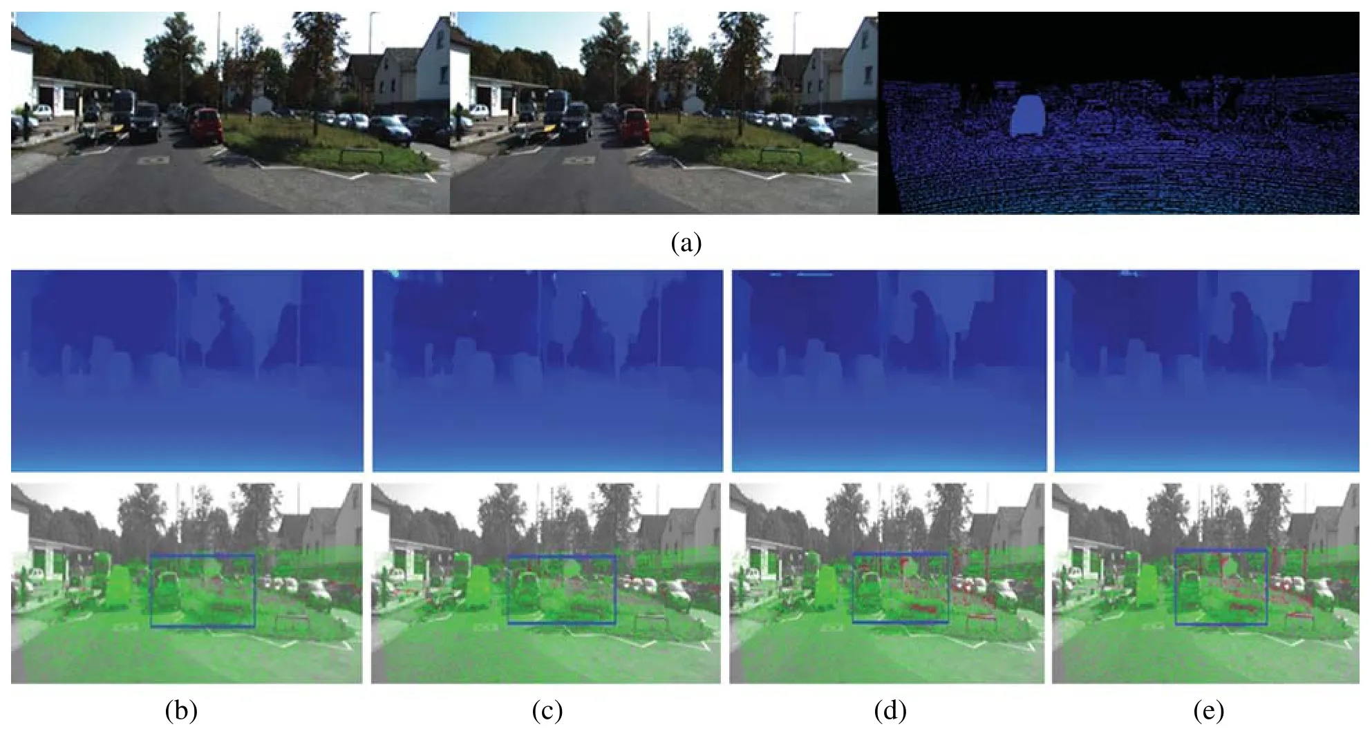
Figure 9:Results of disparity estimation for KITTI 2015.(a) The left and right images and the groud truth (b) SAResNet (c) SADenseNet (d) [32] (e) [22]
7 Conclusion
In this paper,a stereo matching method based on the space-aware network is proposed,which can combine the advanced network model with our network model,and then solve the GPU memory limitation problem through a vertical splitting method,and further improve the network performance by using hybrid loss.Our proposed method is trained on KITTI 2012 and KITTI 2015 datasets and compared with other methods.The experimental results show that the proposed method gives a better performance,with an error rate of 1.23% on KITTI 2012 and 1.94% on KITTI 2015.
Funding Statement:This work was supported in part by the Heilongjiang Provincial Natural Science Foundation of China under Grant F2018002,the Research Funds for the Central Universities under Grants 2572016BB11 and 2572016BB12,and the Foundation of Heilongjiang Education Department under Grant 1354MSYYB003.
Conflicts of Interest:The authors declare that they have no conflicts of interest to report regarding the present study.
杂志排行
Computer Modeling In Engineering&Sciences的其它文章
- Nonlinear Problems via a Convergence Accelerated Decomposition Method of Adomian
- Exact Run Length Evaluation on a Two-Sided Modified Exponentially Weighted Moving Average Chart for Monitoring Process Mean
- An Effective Feature Modeling Approach for 3D Structural Topology Design Optimization
- Three-Dimensional Modeling of the Retinal Vascular Tree via Fractal Interpolation
- Experimental and Numerical Study on the Shear Strength and Strain Energy of Rock Under Constant Shear Stress and Unloading Normal Stress
- Eliciting Requirements from Stakeholders’Responses Using Natural Language Processing
