Impact of climate-smart agricultural technology on multidimensional poverty in rural Ethiopia

Department of Economics,College of Business and Economics,Arsi University,Assela 2120,Ethiopia

Abstract A large body of empirical literature showed that the adoption of agricultural technologies reduces poverty. However,dominants of those studies so far used one-dimensional income or expenditure-based measures of poverty which may not reflect other types of deprivations. Therefore,the major objective of this study is to examine the impact of adopting climate-smart agricultural technology,which refers to a joint application of row planting methods and the use of chemical fertilizers,on the multidimensional poverty status of rural households in Ethiopia. To estimate the impact of the stated technologies,this study employs propensity score matching and endogenous switching regression methods. To measure the multidimensional poverty index,the study also uses the Alkire and Foster counting approach. Using the Ethiopian Socioeconomic Survey (ESS),collected in 2015-Wave 3,the results of the study show that the adoption of these technologies reduces deprivation score and one of its component,the standard of living part. Regionally,a high reduction in deprivation is observed in Amhara and Oromiya regions. The results also show that the impact is significantly higher in severely deprived households. It is also observed that the reduction in multidimensional poverty due to the technology is through an increase in income/consumption via improvement in production gain. The impact channels more through the non-food expenditure pathway. Finally,this study also sheds light on the effects that technology adoption has on multidimensional poverty reduction.

Keywords:multidimensional poverty,rural poverty,technology adoption,poverty reduction,poverty pathways,Ethiopia

1.Introduction

Over the last few decades,the global poverty rates have declined noticeably,nonetheless,the number of people still living in extreme poverty (below 1.90 USD per capita per day) remains high (World Bank 2017). In sub-Saharan Africa (SSA),about 413 million people are living in extreme poverty in 2015 (Beegleet al.2016),and the number of poor has increased significantly since the 1990s and about 88% of the world poorest are expected to live in Africa by 2030 (World Bank 2015a). In Ethiopia,a substantial number of the rural population lives below the national poverty line (33%),and an additional 14% of nonpoor households are estimated to be vulnerable to falling into poverty (World Bank 2015b). The country is among the poorest nations in the world,is highly drought-prone,and has an agricultural sector that accounts for about 85%of employment (Spielmanet al.2010; Derconet al.2012).As there is a stagnant growth of the agricultural sector and persistent food insecurity in low-income countries -notably in SSA1In much of SSA,the agricultural sector is a key fundamental for improving economic growth,overcoming poverty,and enhancing food security,as well as price control in an excess demand situation. However,the sector is mostly dominated by the low use of modern technologies and low productivity (Asfaw et al. 2012b). This being the case in this region,one of the possible solutions for fighting poverty is through improving productivity,profitability,and sustainability of smallholder farming (World Bank 2008). Besides,highly productive agricultural sector facilitates the allocation of resources to other sectors,services,and industry,while at the same time maintaining a better-balanced economy.-there has been continued interest in the adoption of new technology and its impact on productivity in these regions,where climate change further imposes threats to the agriculture systems in general. Thus,modern agricultural technologies can improve household welfare status under climate variability by increasing agricultural income (Wainainaet al.2018) through some mechanisms like higher yields or lower production costs or even by saving labor for alternative economic activities.

Hence,the eradication of poverty continues to be a top priority on the international development agenda. Many of the world poor are smallholder farmers who depend on agriculture as the main source of food,income,and employment. Agricultural growth and development,and the consequent reduction of poverty and its dimensions,are not possible without yield-enhancing technological options because,except in a few areas and under limited circumstances,it is no longer possible to satisfy the growing demands of increasing populations by expanding areas under traditional cultivation. Several studies indicate that agricultural development is one of the main pathways for poverty alleviation (de Janvry and Sadoulet 2009; World Bank 2015a); such that the development and dissemination of improved agricultural technologies such as crop varieties and complementary agronomic practices are major drivers of smallholder welfare improvement in general and the agricultural productivity growth in particular (Aleneet al.2009; Suri 2011; Zenget al.2015;Abdoulayeet al.2018; Kassieet al.2018).

Modern and new agricultural technologies and improved practices play a prominent role in increasing agricultural production and hence improving national food security thus reducing poverty in developing countries,and in general,enhance the overall growth (Kassieet al.2011). When technologies are successfully adopted,the potential impacts go to overall economic growth performance and positively affects natural resources as well (Faltermeier and Abdulai 2008; Sanchezet al.2009).

From the empirical inquiry,quite a lot of studies have presented that the adoption of improved agricultural technologies generally has positive effects on farmers’welfare. If technologies are successfully adopted,they reduce poverty (Becerril and Abdulai 2010; Kassieet al.2011; Asfawet al.2012b; Khonjeet al.2015;Zenget al.2015; Verkaartet al.2017; Habtewold 2018;Mandaet al.2019; Wossenet al.2019; Biruet al.2020).Specifically,the adoption of some specific improved varieties significantly increases yield (Villanoet al.2015;Zenget al.2015; Khatun and Haider 2016; Tufaet al.2019),rise crop and household income (Kassieet al.2011; Bezuet al.2014; Khonjeet al.2015; Verkaartet al.2017; Mandaet al.2019; Tufaet al.2019),increase consumption (Becerril and Abdulai 2010; Asfawet al.2012a,b; Mulugeta and Hundie 2012; Bezuet al.2014;Wordofa and Sassi 2020; Habtewold 2021),improve child nutrition (Kabungaet al.2017; Zenget al.2017;Habtewold 2021),and dietary diversity (Kabungaet al.2017; Teklewoldet al.2019; Wordofa and Sassi 2020).

Hence,the path out of the poverty trap in low-income nations depends on the growth and development of their economically dominating agricultural sector for several reasons,it alleviates poverty through income generation and employment creation in rural areas; helps meet growing food needs driven by rapid population growth and increased welfare and consumption; keeping food prices low,both for urban households stimulating overall economic growth in agriculture-based economies; and conserving natural resources (Kassieet al.2010).

But,one of the big puzzling phenomena in SSA is the low and incomplete/discontinued adoption rate of seemingly profitable technology (Sheahan and Barrett 2017; Macours 2019). One of the major questions that the literature on technology adoption needs to enquire about is whether accurately productive and profitable technologies are available in SSA and other low-income countries. Related to this issue it is also important to identify the appropriate agricultural technologies that can bring about significant and sustainable improvement in productivity in regions like SSA.2In a region where agriculture is a predominant sector that underpins the livelihoods of most of the poor,adopting more technologies like high yield varieties (HYVs),and associated products such as crop insurance contribute to economic growth and poverty reduction among rural societies and the poor (Kelsey 2011). According to Ravallion et al. (2007),many poor households in SSA and South Asia live in rural areas where farming is their only livelihood. Their study also shows that almost 75% of those living on less than a dollar per day will remain in rural areas till 2040. Similarly,Mendola (2007,p.373) states,“of the poor people worldwide (those who consume less than a ‘standard’ dollar-a-day),75% work-and live-in rural areas. Projections suggest that over 60% will continue to do so in 2025.” Thus,there is a direct link between poverty reduction and increasing agricultural productivity. This can also create employment opportunities for landless wage laborers.

Similar to other SSA countries,Ethiopia’s population is increasing dramatically,expected to grow to 160 million by 2050 (Josephsonet al.2014) which exacerbates the situation of extreme poverty and food insecurity. On the other hand,due to population growth and other related factors farm sizes have been rapidly declining,increasing the need for agricultural intensification (Headeyet al.2014) and search for better agricultural technology.Thus,among others,rising the agricultural outputs of smallholders through improved technology is one of the policy priorities for development agencies and the Ethiopian government (Abebaw and Haile 2013).

From the measurement sides,however,most existing welfare studies argue that poverty has always been understood as a multidimensional problem especially since Sen’s (1976) work,even if most of the poverty studies still measure poverty using a one-dimension -income or expenditure-based -approach. According to Alkire and Foster (AF) (2011b) “how we measure poverty can importantly influence how we come to understand it,how we analyze it,and how we create policies to influence it. For this reason,measurement methodologies can be of tremendous practical relevance.”

A traditional mechanism for measuring poverty,the standard of living,or quality of life is based on a household unit’s aggregate value of a single indicator,monetary income,or on its consumption levels (Alkire and Sarwar 2009). In this approach,a person is defined as poor if his/her income is below a certain per-determined poverty line,however,this method (unidimensional approach of poverty) can be used when a well-defined unidimensional indicator such as income,is identified as the basis for poverty evaluation (Alkire and Foster 2011b). The simplistic assumption,in this case,is that the single-dimensional indicator variable has a cardinal nature; however,in some cases,the variable may only have ordinal significance (that is,the direction of change is discernable,but not its magnitude).

However,over time there has been growing consensus regarding the insufficiency and incompleteness of income poverty measures (Sen 1992). The first thing to note here is that some important welfare components (poverty status indicators in our case) are not satisfied in the market or that markets function very imperfectly. The second thing is that each household has a different capacity to convert income into heterogeneous functioning which leads to differing welfare status among households. As Alkire and Santos (2013) argued the third is,“participatory exercises reveal that poor people describe their state of deprivation using a wide range of dimensions including health,nutrition,lack of adequate sanitation and water,social exclusion,low education,bad housing conditions,violence,shame,and disempowerment. Fourth,income is merely a means to an end. It is the end,which is valuable,not the means.” Identifying the poor and checking whether a person meets a set of minimum basic needs or not is the dominant task. Since Sen’s(see 1976,1979,1985,1987,1992,and 1995) influential work,poverty has been increasingly recognized as a multidimensional phenomenon. Many factors other than income can provide important information on wellbeing and poverty such as the state of health,the level of education,ownership of assets,and access to basic services.3See the works (Tsui 2002; Atkinson 2003; Bourguignon and Chakravarty 2003; Alkire and Foster 2007,2011a,b,2016; Alkire 2011;Battiston et al. 2013; Alkire and Santos 2014; Alkire et al. 2015; Maasoumi and Xu 2015) for further discussion of multidimensional poverty and its natures in detail.

There are,however,large bodies of well-established empirical literature that shows adopting agricultural technologies reduces poverty and food insecurity,leads to an increase in household incomes,raises productivity,gives more opportunities for market access,and leads to an overall increase in social welfare measured by monetary income or expenditure-based approaches (e.g.,Mendola 2007; Adekambiet al.2009; Becerril and Abdulai 2010; Kassieet al.2010,2011; Asfawet al.2012b;Khonjeet al.2015; Zenget al.2015; Verkaartet al.2017;Habtewold 2018; Mandaet al.2019; Wossenet al.2019;Biruet al.2020).4A few studies have analyzed the effects of some improved practices and interventions on multidimensional poverty (Bucheli et al.2016;Pasha 2016; Ogutu and Qaim 2019),but not the impact of climate-smart agriculture on multidimensional poverty.They assessed impacts of different improved agricultural technologies and found that those technologies reduce poverty in general. Nevertheless,all these studies use income or expenditure-based measures of poverty,which may not reflect other types of deprivations as poverty is a multidimensional phenomenon.5Yet,several existing studies on poverty effects of improved agricultural technologies only looked at income poverty data. Even though income (or expenditure) data are extensively used to analyze poverty,they cannot fully capture the multidimensional nature of poverty,including deprivations in education,health,nutrition,and other dimensions of living standard. The simple assumption that additional income earned due to the use of improved agricultural technologies will automatically be spent on satisfying basic needs may not always be true. Different types of income may be controlled by different persons within the farm household and used for different purposes (Meemken et al. 2017) and each household has a different capacity to convert income into heterogeneous functioning which leads to differing welfare status among households.

Alkire and Foster (2007) argued,“income and consumption indicators reflect material resources that are vital for people’s exercise of many capabilities. The use of monetary indicators alone,however,often reflects an assumption that these indicators are good proxies for multidimensional poverty. But monetary poverty often provides an incomplete measure of poverty and insufficient policy guidance regarding deprivations in other non-monetary dimensions.” Nowadays,there is a renewed interest in a multidimensional approach to poverty since relevant databases are increasingly available which enable comparative methodological and empirical analyses (Batana 2008),and many studies contribute to the debate on the relative importance of‘direct’ and ‘indirect effects’ of adopting agricultural technologies within poverty alleviation strategies,however,studies miss many important aspects of poor people’s lives including the diverse ways in which technology directly or indirectly affects their livelihoods.

Coming back to the technologies,the original articulation of the concept climate-smart agricultural technology (CSAT hereafter) was presented in the FAO(2009) report. The following year FAO’s paper (FAO 2010) defines climate-smart agriculture as “agriculture that sustainably increases productivity,enhances resilience,reduces greenhouse gases,and enhances achievement of national food security and development goals”. The idea reflects a motivation to progress the integration of agriculture development and climate responsiveness. The notion of CSAT emerged as a promising way to secure food for the fast-growing world population under climate change conditions (McCarthyet al.2011). It aims again to achieve food security and broader development goals within the context of a changing climate and increasing food demand (Lipperet al.2014). The CSAT includes both traditional and innovative practices and technologies that promote agricultural productivity and generate income for the growing population.

Adoption of CSAT is an improved practice and approach for transforming and reorienting agricultural systems to ensure food security status of people and fight malnutrition under climate change and variability. Its adoption has also the potential to increase agricultural productivity and enhance farmers’ sustainable livelihoods and resilience to climatic shocks (Fentie and Beyene 2019). It is also one of the best ways to alleviate poverty and boost food security through enhanced agricultural productivity and incomes of farm households in lowincome regions like Africa (James and Jones 2015);supports food security under climate change through its three goals:(1) improve agricultural productivity; (2) build resilience to climate change; and (3) reduce agricultural greenhouse gas emissions (Lipperet al.2014).

In the case of Ethiopia,CSAT and practice is actively promoted to farmers for many decades (Jirataet al.2016)and its practice ranges from the farm level to international policy and financial mechanisms (Fentie and Beyene 2019). Row planting is one of the labor-intensive CSAT and practices (Vandercasteelenet al.2014; Dinku and Beyene 2019). Thus,the current study focuses on the joint impacts of row planting with chemical fertilizer at country level.

This research,thus,contributes to a growing literature by exploring the impacts of CSAT on multidimensional poverty,in which much of the previous work has focused on the impacts of improved agricultural technologies on several welfare indicators without assessing the effects on multidimensional poverty. Again,to the best of the researcher’s knowledge,this is the first study assessing the role of CSAT on the multidimensional poverty status of rural households in Eastern Africa and Ethiopia.The empirical question that this research address is:does CSAT have the potential to affect households’multidimensional poverty status? If yes,under what circumstances?

Through the review of the vast literature,it was also observed that most previous studies on the adoption and welfare impacts of CSAT have focused on the impact of a single agricultural technology,though,farmers are faced with a bundle of improved technologies that may be adopted in combination,with complementary effects (Moyo and Veeman 2004; Teklewoldet al.2013; Teklewoldet al.2017; Wainainaet al.2018). Thus,the study also contributes to the literature such that it considers combined sets of modern agricultural technologies and improved practices,and their welfare impacts.

Specifically,the study compares the results of measuring multidimensional poverty with those of standard unidimensional approaches for measuring poverty which is based on consumption measures,and considers whether the inclusion of additional dimensions leads to a change in a household’s poverty level from the standard-based approach. It also accounts for other issues such as weighing the dimensions of poverty used in its aggregation.

The rest of the paper is organized as follows. Section 2 describes the methodology used for estimating multidimensional poverty and the impact of the stated technology. Section 3 discusses the findings of the study. Section 4 gives the concluding remarks and policy implications.

2.Methodology

2.1.Theoretical framework and empirical strategy

Theoretical framework of the decision to adopt agricultural technologiesAgricultural households(farmers) have to face the outcomes of adopting new and improved production technologies that are uncertain(Rahm and Huffman 1984). Thus,the decision to adopt CSAT can be modeled in a random utility framework following the literature (e.g.,Becerril and Abdulai 2010; Di Falcoet al.2011; Kassieet al.2011; Shiferawet al.2014;Khonjeet al.2015). Hence,it is assumed that farmer households take adoption decisions6In this study,an adopter is defined as a farm household who planted either improved or local (traditional) seeds in recommended spacing (row planting) with chemical fertilizer and a non-adopter is defined as a farmer who did not use the row planting method and chemical fertilizer jointly (in combinations).(which refer to a joint application of row planting methods and the use of chemical fertilizers) based on utility maximization motives.

LetD＊denote the difference between the utility from adoption(U1i)and the utility from non-adoption(U0i)of CSAT,such that a householdiwill choose to adopt the CSAT ifThe two utilities are unobserved and unavailable; but they can be expressed as a function of observable components in the latent variable model so that a linear relationship can be specified for theith farm household between the utility derived from theith technology and observed farm-specific characteristics as:

whereDis a binary 0 or 1 dummy variable for the use of the CSAT;D=1 if the technology is adopted andD=0 otherwise.αis a vector of parameters to be estimated,Zis a vector that represents multidimensional household and farm-level characteristics,andεis the random error term. The two utilities are non-observable and the net benefit (the difference between the two utilities),Di,that a farmer gains from adopting is a latent variable determined by observed and unobserved characteristics defined in eq.(1).

Measuring unidimensional povertyTo assess the impacts of CSAT on households’ standard poverty level,the study uses 12-month consumption expenditure data.The national poverty line developed by MFED (2012)is used to estimate the poverty index. To explore the extent of unidimensional poverty and compare it with multidimensional poverty the study uses a more general class of poverty measurement approach proposed by Fosteret al.(1984) which is easily decomposable into different sub-groups.

Now,let the dimension indicator variable of householdibeyiandzbe the poverty line,whilenandqstand for the total population and the total number of poor in the population respectively,andαis the poverty aversion parameter. Then the unidimensional poverty index,pα,can be expressed as:

whenα=0,p0is simply the headcount ratio,the proportion of people at and below the poverty line. The deprivation vectorg0substitutes each dimensional indicator’s variable at and below the poverty line with 1 and replaces the nonpoor with 0. Ifα=1,p1is the poverty gap index (or depth of poverty),defined by the mean distance to the poverty line where the mean is formed over the entire population with the non-poor counted as having a zero-poverty gap. Then the normalized gap vectorg1replaces each poor income dimensional indicatoryiwith the normalized gap (z–yi)/zand assigns zero to the rest. Finally,whenα=2,p2is the squared poverty gap (severity of poverty index). The squared gap vectorg2replaces each poor dimensional indicator with the squared normalized gap[(z–yi)/z]2and assigns zero to the rest.

Measuring multidimensional povertyFor measuring multidimensional poverty this study uses Alkire and Foster’s (2007,2011a) counting approach which follows the method of aggregation proposed by Fosteret al.(1984),Foster Greer Thorbecke (FGT),which is built on the same family of measures. This family satisfies a certain number of axioms such as decomposability.Following this framework,a counting approach of multidimensional poverty can be developed as follows.

Consider a population ofnindividuals. Letd≥2 be the number of dimensions andx=[xij] then×dmatrix of achievements,wherexijis the achievement of individuali(i=1,...,n) in dimensionj(j=1,...,d).xhas the following form:

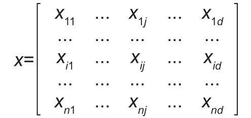
In this case,it should be noted that each row vectorxirepresents individuali’s achievements,while each column vectorxjgives the distribution of dimensionj’s achievements across the set of individuals.

Let |zj|＞0 be the indicators’ cut-off below which a person is deprived in indicatorj.xiis the row vector of individuali’s achievements in each dimension,andxjis a column vector of dimensionjachievements across the set of individuals; thusxijis the achievement of individualiin dimensionj.

Identification of the Poor Sen(1976) identified two major issues in the measurement of poverty:the process of identifying the poor and aggregation of information about poverty across society. In this regard,a relatively easy and straightforward income or consumption-based approach identifies who is poor based on information from a single resource variable.An income or consumption poverty line is the level of the dimension indicator variable necessary for purchasing a basic basket of goods and services,which divides the population into poor and non-poor. In the multidimensional context,however,identifying the poor is more complex than the single dimension approach(Alkire and Foster 2011a). The AF approach,which this study used,combines a method of identifying the poor based on counting the number of (weighted) deprivations on achievements and a method for aggregation based on an extension of the unidimensional FGT family of measures to the multidimensional context.

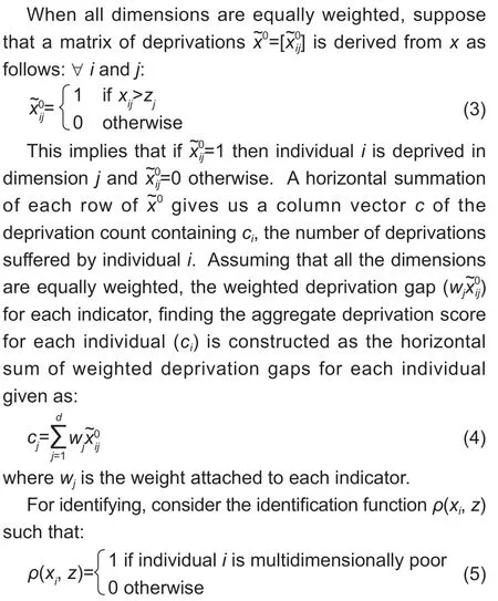
As Alkire and Foster (2007,2011a) explain,there are two identification methods in this poverty analysis:the union and intersection approaches. In the union method,a personiis said to be multidimensionally poor if there is at least one dimension in which the person is deprived(that is,ρ(xi,z)=1 if and only ifci≥1). The intersection method,which identifies personias poor only if the person is deprived in all the variables of the dimension indicator (that isρ(xi,z)=1 if and only ifci=d). However,both methods have their shortcomings. A normal and reasonably good approach to identify the poor is using a value of the cut-off level forcithat ranges somewhere between the two extremes of 1 andd. Letkbe the cutoff (a value ranging from the minimum weight assigned to any indicator,union criterion,to the total number of considered indicators,the intersection criterion).

An equal weight is assigned across dimensions and the same weights to all indicatorsjwithin each dimension.This was done by assuming that the available selected dimensions are relatively equally important (Alkire and Foster 2011a). Next,the multidimensional poverty index(MPI) for both the poor and non-poor households is computed following the Alkire and Foster (AF) (2007,2011a) methodology.

The multidimensional poverty measuresletM(x;z) be the class of multidimensional poverty measures proposed by Alkire and Foster (2007). Applying the method proposed by the AF family of multidimensional poverty,we have two basic parts to be computed:the first measure is given by the headcount ratio (H),which is the proportion of incidence (depth) of people who experience multiple deprivations and is gives as:

And the average deprivation shares across the poor by the intensity or breadth of poverty (A) is the average deprivation score of those poor segments of the population:

The second measure combinesHandAto obtain an expression satisfying dimensional monotonicity (unlikeH).The new measureM0called the adjusted headcount ratio is given by the product of the above two terms (H×A) as:

Note also that the remaining classes of multidimensional poverty indices can be computed by simply varying the values ofαin the general setting,Mα(x;z). Whenα=1,the measureM1is called the adjusted poverty gap and ifα=2 the measureM2is called the adjusted squared poverty gap.

Decomposability and dimensional break-down of MPIDecomposability implies that overall poverty is a population share weighted average of sub-group poverty levels. All members of theMαfamily can be disaggregated/decomposed into its components (Alkire and Santos 2013). Thus,overall poverty can be decomposed across different population sub-groups. In this process,each measure (portion of MPI) can be represented as the weighted sum of individual poverty,where each person has a relative weight of 1/n:

So,if we have a population sub-groupI,its contribution to overall poverty can be expressed as:

where (nI/n) andMαare the population share and the poverty measure of sub-groupI,respectively,andMαis the poverty measure of the overall population.7As Alkire and Santos (2013) state,“Whenever a region’s contribution to poverty or some other group widely exceeds its population share,this suggests that there is a seriously unequal distribution of poverty in the country,with some regions or groups bearing a disproportionate share of poverty. The sum of the contributions of all groups needs to be 100%.”

2.2.Empirical strategy

This study employs a combination of methodologies to ensure the consistency of its results and for checking the robustness of its empirical findings. Both propensity score matching (PSM) and endogenous switching regression(ESR) methods are employed to evaluate the impact of CSAT on multidimensional poverty. The heterogeneity in the decision to adopt or not to adopt a new agricultural technology and the unobservable characteristics of farmers and their farms are controlled by estimating a simultaneous equations model with endogenous switching using the full information maximum likelihood (FIML)estimation method. The non-parametric regression method,PSM is also used for assessing the robustness of the results.8The researcher advises interested readers refer to Rosenbaum and Rubin (1983); Caliendo and Kopeinig (2008); Becerril and Abdulai(2010); Kassie et al. (2011) for PSM and Lokshin and Sajaia (2004); Di Falco et al. (2011); Shiferaw et al. (2014); Khonje et al. (2015)for ESR.

The propensity score is defined as the conditional probability of receiving a treatment given pre-treatment characteristics as:

whereDi={0,1} is the indicator of exposure to treatment andXis the multidimensional vector of pre-treatment characteristics.

In this case,if the exposure to treatment is random within cells defined byX,it is also random within cells defined by the values of the mono-dimensional variableP(X) (Rosenbaum and Rubin 1983). As a result,given a population of units denoted byi,and if the propensity scoreP(Xi) is known,then the average treatment effect on the treated (ATT) can be estimated as:

whereY1iis the outcome for the treated group andY0ifor the non-treated group. To assess the consistency of the results under different assumptions,this study also uses the ESR techniques. Let household welfare be indicated by “multidimensional poverty status”Y1ifor adopters andY0ifor non-adopters. The endogeneity of the adoption decision is accounted for by estimating a simultaneous equations model with endogenous switching using the FIML estimation method. The selection equation for technology adoption is specified as:

wherethe unobservable or latent variable for technology adoption andDiis its observable counterpart.

To account for sample selection biases this study uses an ESR model of welfare outcomes where farmers face two situations:(1) adopting a CSAT,and (2) not CSAT/continuing using the old technology. This is defined as:

whereYi,is outcome variables,the multidimensional poverty status of households in regimes 1 and 2,Xirepresents a vector of exogenous variables thought to influence the multidimensional poverty status of households. Thus,eqs.(12a) and (12b) describe the relationship between the variables of interest in each of the two regimes. But the model must be correctly identified. For the model to be identified,the issue of exclusion restrictions is important (Di Falcoet al.2011),in which the selection instruments,not only those automatically generated by the non-linearity of the selection model of the technology adoption (eq.(11)) but also other variables directly affect the selection variable while at the same time do/do not affect the outcome variable(s) (Appendix A).

In the literatures (e.g.,Di Falcoet al.2011; Shiferawet al.2014) stated that the error terms in eqs.(11),(12a),and (12b) are assumed to have a trivariate normal distribution with mean vector zero and covariance matrix:

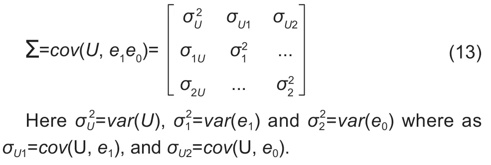
The ESR framework can be used for estimating the average treatment effect of the treated (ATT) and of the untreated (ATU),by associating the expected values; e.g.,see Khonjeet al.(2015),ATT and ATU are calculated using the following framework:

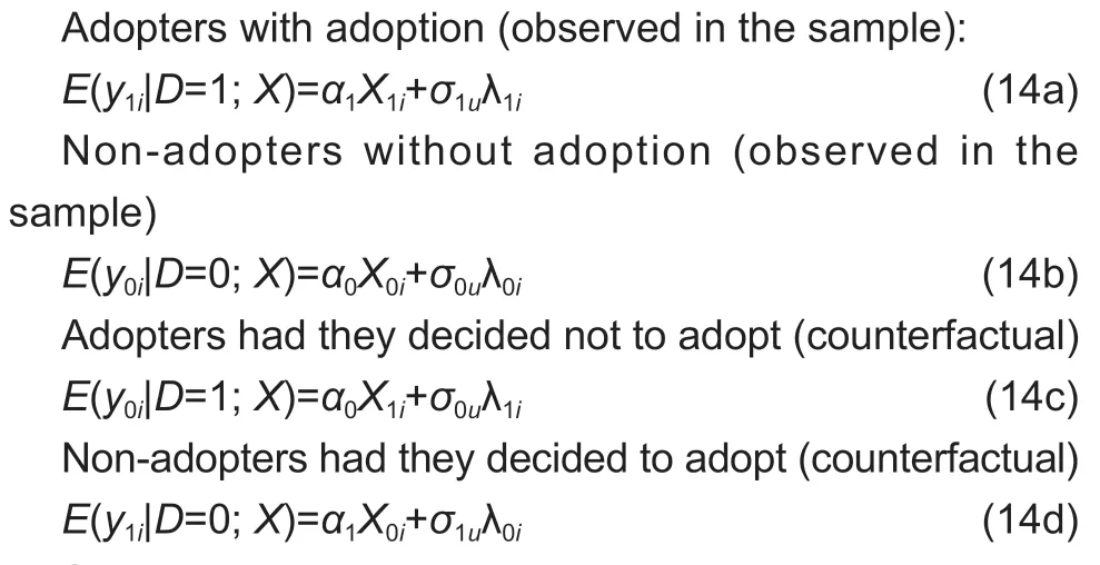
SinceY1iandY0iare not observed simultaneously the covariance betweene1iande0iis not defined (Maddala 1983,p.224; Lokshin and Sajaia 2004). An important implication of the error structure in the ESR approach is that because the error term of the selection eq.(11)uiis correlated with the error terms of the outcome eqs.(12a)and (12b) (e1iande0i),the expected values ofe1iande0iconditional on the sample selection are nonzero (Di Falcoet al.2011);where λ1iand λ0iare the inverse Mill’s ratios (IMRs)computed from the selection eq.(11),and we include them in eqs.(12a) and (12b) to correct for selection bias in a two-step estimation procedure.

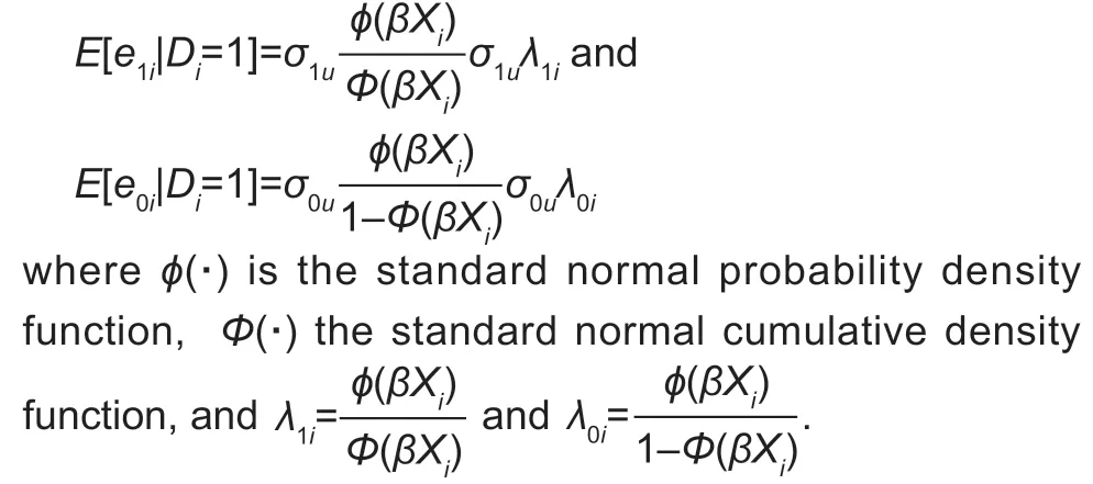
Eqs.(14a) and (14b) represent the actual expectations observed from the sample,while eqs.(14c) and (14d)are the counterfactual expected outcomes. The ATT is computed as the difference between eqs.(14a) and (14c)as:

Similarly,the expected change in non-adopter’s multidimensional poverty status had they been treated,which is the ATU is given by the difference between eqs.(14d) and (14b) as:

2.3.Data sources and measurement of key variables

This study uses data from Ethiopian Socioeconomic Survey (ESS),a nationally representative survey of rural households of Ethiopia from 2015-Wave 3,collected under the Living Standards Measurement Survey-Integrated Surveys on Agriculture (LSMS-ISA) of the World Bank in collaboration with the Central Statistical Authority (CSA).The data targeted the rural parts,small and medium towns in the country,however,households from both small and medium towns were excluded because of the non-applicability of agricultural technology adoption after which the sample size becomes 3 727. After adjusting and accounting for missing variables and values,the final sample used in the study is 2 752 households for which complete data are available. The dataset has good qualities as it contains information regarding income or consumption expenditure,so we can assess how the inclusion of additional dimensions of poverty affect our measurement of poverty following the MPI approach and comparing this with the monetary approach.

The focus of this study is to explore the impact of CSAT on multiple rural dimensions of poverty. Unfortunately,the data do not contain information on the health dimension attributes of child mortality and nutrition. To address this problem,we use parental consultation and physical or mental disability indicators to represent the health dimension. Similarly,there is no information on one indicator of education,child school attendance,in the dataset so we also use the reading and writing abilities of any household member as a possible proxy. The outcome variables of interest in our study are the composite MPI score and its three dimensions. We compute these values by following the methodology developed in Alkire and Foster (2007,2011a). The multidimensional index ranges between 0 and 1,where 1 means total deprivation in every indicator and 0 denotes no deprivation in any indicator. The index is computed with a bundle of equallyweighted dimensions -health,education,and living standards -sub-divided into 10 indicators in our case,but the number of dimensions or indicators can vary based on objectives and other interests (Table 1).

3.Results and discussion

3.1.Descriptive analysis

In this section,the study reports and discusses the descriptive statistics of poverty analysis. The first part presents a unidimensional measure which is followed by a descriptive statistical analysis of poverty using different multidimensional poverty estimation results at the household level.

The study uses consumption expenditure in the unidimensional approach and the poverty analysis is done at the household level. The national poverty lines developed by MFED (2012) is used to estimate the poverty index. The estimated result of consumption expenditure-based poverty analysis shows that about 42%of the households are poor in the country (Appendix B).

Concerning the adoption status of households,adopters of CSAT are slightly better off than the nonadopters. The incidence of poverty is higher among non-adopters (42.1%) than among adopters (41.6%)which implies that adopters are better-off due to the‘technology impact’. A comparison between sexes also shows that female-headed households are relatively less impoverished than male-headed ones. This result shows that 42.3% of male-headed households are under poverty while only 40.1% of the female-headed households are impoverished.

A region-wise comparison also shows that the status of poverty differed from one region to the other ones.Benishangul is the most impoverished region (59%)followed by SNNP (57.1%),and Amhara (49.5%). On the other hand,in Dire Dawa,the incidence of poverty is the lowest (3.30%) followed by Harari (14.2%). These poverty levels are much higher than the national poverty rate;the government’s official report maintains that nationally the incidence of poverty is only about 24% in 2015–2016(MFEC 2017).

To consider heterogeneity among different social groups,mainly differentiated by adoption status,gender,and region (geographical location),a heterogeneous poverty line is constructed using the median of consumption expenditure. The estimated poverty based on an analysis of the relative poverty line shows that about 47.2% of the households are poor. This result shows that more poor were found using the relative poverty line as compared to the results using the absolute poverty line which applies to every group regardless of its initial conditions.

Similarly,comparisons across different groups also shows an increase in poverty when we used the relative poverty line. Example,about 41.6% of the adopters are poor in the case of the absolute poverty line,but this increases to 46.8% when the relative poverty line is applied. Male-headed households’ poverty status increases from 42.3 to 48.2% as a result of using the relative poverty line. Concerning the regional distribution of relative poverty,the Benishangul region has the highest poor population (64.6%) followed by Amhara and SNNP with 57.7 and 56.0% poor population respectively. The high relative poverty rates suggest that high levels of inequalities among people in rural consumption.

For the empirical parts of the analysis (using PSM),it is also important to check the matching quality of the model.Before estimating the causal effects of the technologies,we tested the matching quality. The matching methods were tested,and they passed different quality checking tests. After estimating the propensity scores for the adopter and non-adopter groups,the common support condition was also checked. The standardized bias reduction,joint significance and pseudo-R2tests are used.The covariate balancing tests before and after matching are reported in Appendix C. The standardized mean difference for overall covariates used in the propensity scores for the two outcome variables,the total deprivationscore and the living standards deprivation score,is between 35.2–48.8% before matching,and the value reduces below 5% after matching.

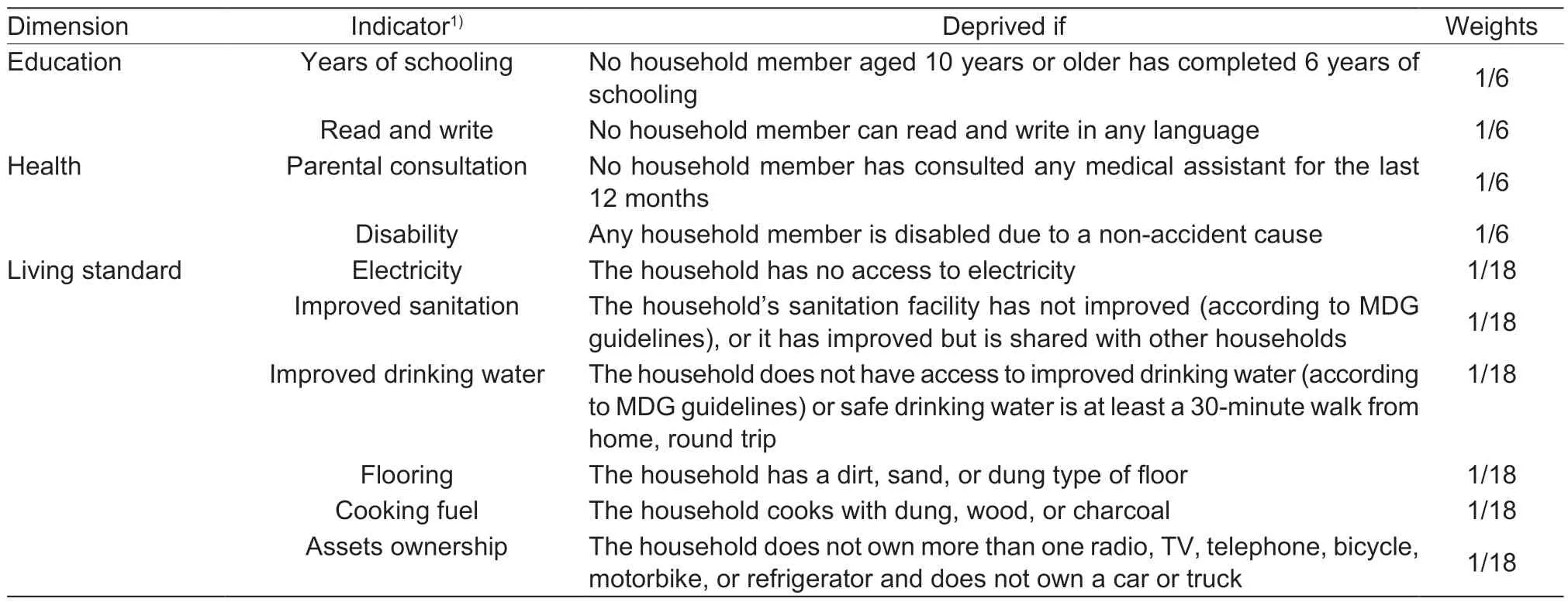
Table 1 Multidimensional poverty index’s (MPI’s) dimensions,indicators,deprivation cutoff,and weights

TheP-values of the likelihood ratio tests show that the joint significance of the covariates is always rejected after matching,whereas it is never rejected before matching. The pseudoR2also drops significantly from around 19.5–20.4% before matching to about 0.1–0.7%after matching under the two outcome variables. The likelihood ratio test is also statistically significant before matching but becomes insignificant after matching. The low pseudoR2,high bias reduction,and the insignificantP-values of the likelihood ratio test after matching suggest that the proposed specification of the propensity score is successful in terms of balancing the distribution of covariates between the adopter and non-adopter groups.

After this review and description of the state of conventional poverty levels of households in different categories,we present the multidimensional poverty status of households disaggregated into different household groups. The study uses the AF’s three dimensions and 10 indicators approach for estimating different forms of multidimensional poverty indices. Table 2 gives a summary of MPI’s dimensions and indicators for the entire sample. The results show that people are the most deprived in the education dimension (41.8%) followed by the standard of living dimension (34.6%). Indicatorwise,people are the most deprived in terms of years of schooling (24.6%) while they are less deprived of access to clean water (3.2%).

Table 3 below also presents the MPI for different household groups (decompositions). One of the advantages of using MPI for measuring poverty is that it can be disaggregated into different household groups,dimensions,or indicators. First,results are disaggregated into adopter and non-adopter categories,then by sex,and finally by region.

The results in Table 3 show that the adopters are less deprived in all the dimensions,except health status,implying that adoption of CSAT improves social welfare(even though a further evaluation of the actual impact needs to be done). The estimated multidimensional headcount ratio (H) and the adjusted multidimensional headcount ratio (Mo) are reported for both adopters and non-adopters and the results are almost similar for the two groups with a slightly higher poverty rate for nonadopters in terms of adjusted multidimensional headcount ratio (59.8%) as compared to 56% for the adopter group.

When it comes to the contribution of each dimension,the results also show that both adopter and non-adopter households are most deprived in the education dimension while health deprivation is the lowest in both categoriessupporting the results of the entire sample (also see Fig.1 below where the results are disaggregated by gender).

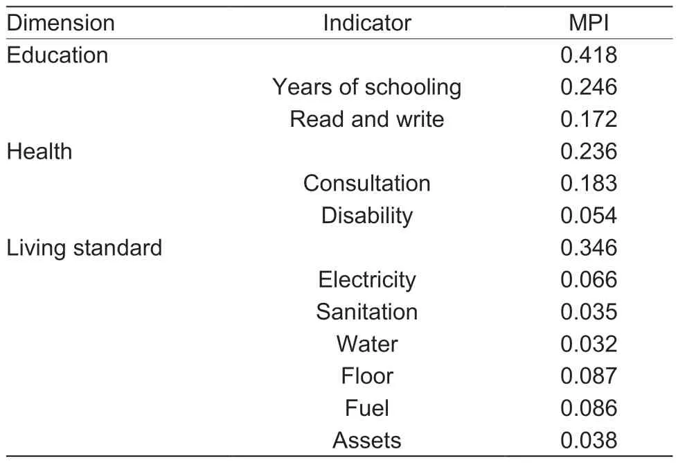
Table 2 Summary of multidimensional poverty index’s (MPI’s)dimensions and indicators

The analysis on male-and female-headed households also shows that gender differences in poverty status are significant. Male-headed households are less deprived as compared to female-headed ones in both the multidimensional headcount ratio (94.75%vs.97.4%)and the adjusted multidimensional headcount ratio(56.6%vs.66.0%). In terms of the contributions of each domain,like the cases observed earlier,the education dimension shows higher differences between maleand female-headed households. Fig.1 also shows the contribution of adopters and non-adopters to aggregate MPI disaggregated by sex,and the results support the findings presented in Table 3,indicating that both adopter and non-adopter categories have almost similar status of poverty in most cases.

Looking at the health dimension,male-headed households register a higher MPI than female-headed households. The basic reason for female-headed households having a low MPI as compared to the maleheaded group in the health dimension is that the current national health policy focuses on women and children’s healthcare. This result supports conventional poverty outputs where female-headed households register lower values in the headcount index.

Concerning the standard of living component of MPI,male-headed households contribute more to poverty.As can be seen from Table 3,about 36% of them are deprived in the standard of living,while femaleheaded households are slightly less deprived (31.2%).Table 3 also shows that female-headed households have better access to asset holdings.

The third disaggregation that the research follows is the decomposition of MPI by regions in the country(see Table 4). To acknowledge the advantages of the multidimensional poverty approach,MPI’s regional disaggregation is performed. A closer look at the adjusted multidimensional headcount ratio (Mo),under the indices in the sub-group column,shows that the three most deprived regions are Somalie,Afar,and Amhara with Mo values of 66.2,65.8,and 63.7 percentage points,respectively.

Except for these three regions,on average,the adjusted multidimensional headcount ratio is almost equally distributed among the remaining seven regions.In terms of contribution to overall poverty in the country,the highest proportional poverty is registered in SNNP followed by Amhara and Oromiya regions. Except for SNNP,Amhara,and Oromiya the remaining regions have a small number of inhabitants and makes a small contribution to aggregate poverty. Like the results given in Table 4,Appendix D also shows the contribution of each component of MPI in the aggregate deprivation score in each of the 10 regions and the results support the findings reported in Table 4.

In the descriptive analysis,the study compares the conventional approach to multidimensional approaches.More deprived households are found following the multidimensional approach (58.6%) as compared to the consumption-based absolute poverty approach (42%)using the absolute poverty line; while the proportion of the poor increases to 47.2% when the relative poverty line is used. Thus,the descriptive analysis show that the way we measure poverty matters for the status of the poor.

3.2.Econometric results

Like the descriptive section,this econometric section starts with an analysis of the conventional povertyapproach. Each estimated effect of the CSAT is reported in both aggregate and decomposed ways. Once we have estimated the propensity scores and checked their matching quality,we compute the ATT of the outcome variables,consumption expenditure,and headcount ratio,for comparing these with the multidimensional approach to poverty,which is the main interest of this research. Four commonly used matching algorithms are employed -the nearest neighborhood matching (NNM),kernel-based matching (KM),radius matching (RM),and stratified matching (SM). The estimated results based on the first three matching algorithms are reported in Table 5.The results show that the adoption of CSAT has a positive and significant effect on consumption expenditure and a negative impact on poverty as measured by the headcount ratio.

Table 3 Multidimensional poverty index’s (MPI’s) dimensions and indicators (by sub-groups)

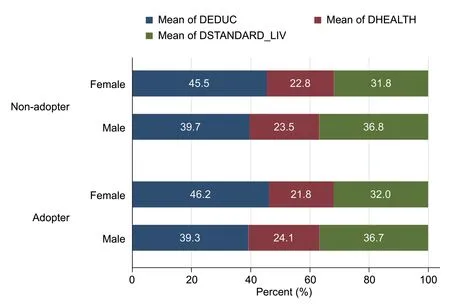
Fig.1 Contribution of each multidimensional poverty index (MPI) domain to total deprivation across adoption categories by sex.DEDUC,DHEALTH,and DSTANDARD_LIV stand for education,health,and living standard deprivations,respectively.

The average welfare (per capita consumption expenditure) gains of CSAT range from 152 ETB to 203 ETB under the three matching methods and the estimated gains are statistically significant. The estimated results measure the average differences in consumption expenditure of the same pairs of households in all pre-treatment characteristics,but having different technological statuses based on adopting and notadopting the CSAT. The impacts of technology adoption on poverty reduction as measured by the headcount index ranging between 0.20–0.31% are all statistically significant. The estimated impact on the headcount index is very low which may be due to the fact that the conventional poverty approach cannot reflect the actual impact of the adopted technology on non-monetary welfare gains such as health,quality of life,and education attainments. So,we need an approach that shows the complete impact of technology on social welfare. Here the best alternative is the multidimensional approach to poverty.

In the main part of the analysis,we look at the impact of the CSAT on multidimensional poverty on each of the deprivation indicators -overall,education,health,and living standards. Using eq.(4) the study computes the aggregate deprivation score.9In contrast to some previous studies like Alkire and Santos (2010) and Alkire and Foster (2011),this study does not censor the MPI deprivation scores to zero for those households with a deprivation less than 0.3 to preserve our sample size and reduce data variability.For overall deprivation and each dimension,the study separately estimates the impact of the CSAT on households’ multidimensional poverty using the aggregate deprivation score as an outcome variable using both PSM and ESR models.

Table 6 reports the results of PSM under the three matching methods for the overall (composite)multidimensional deprivation. The ATT term is negative throughout all the matching methods and statistically significant suggesting that adopter households’multidimensional poverty declines between 2.0 and 3.0%.These results remain consistent even when different matching algorithms are used suggesting that there is a negative effect of being an adopter of the specified technology on the multidimensional poverty weighted score and these results underline the robustness of the findings.

The results also show that the adopters are better-off because of the adopted technology as compared to their counterfactual group supporting the descriptive statistics’results,but in the multidimensional approach,the impact is higher and relatively complete in coverage. The possible reason for the higher reduction in poverty in this section is the inclusion of additional indicators of poverty which are not considered in the conventional approach.An interesting point to note here is that when comparing adopter households with non-adopters,it is seen that adopters did better than their counterfactuals in reducing deprivations and,hence improving welfare.

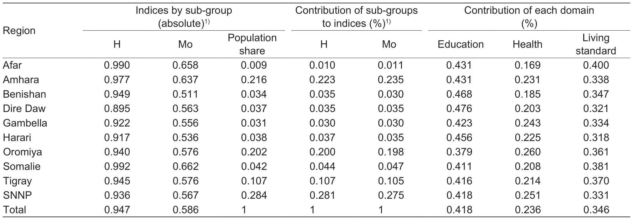
Table 4 Multidimensional poverty index’s (MPI’s) decomposition by regions

Table 5 Impact of technology adoption on unidimensional poverty indicators

As discussed in the previous sections,one of the advantages of using the MPI approach for measuring poverty is that it can be disaggregated (decomposed)into its dimensions and indicators. Appendix E presents the results of the PSM estimation for the living standards dimension. The results show that the adoption of the specified technology is associated with a drop of between 1.6–2.2% in living standards’ deprivation and is statistically significant in all the matching methods. This is consistent with the overall (composite) MPI in terms of both sign and significance,but lower in magnitude in the case of living standards.

Appendix F similarly reports the estimates of MPI’s education dimension. In contrast to the overall and living standard deprivations,here it is observed that adoption of technology is not associated with a statistically significant change in education deprivation,except in the case of radius matching. This situation is repeated for the health dimension in Appendix G which shows that results are similar to the education deprivation such that the association between the adoption and the degree of health deprivation is not statistically significant.

Finally,the impact is disaggregated across regions using the SM method to see the regional differences in terms of deprivation scores and MPI values,and results are reported in Table 7 below. What is more interesting here is that the most productive regions like Amhara and Oromiya register significant reduction in aggregate deprivation scores in all dimensions. This implies that adoption helps the treated group to reduce poverty in thetwo dominant regions in the range 5.4–7.1 percentage points in overall deprivation and 1.6–5.3% in each component of MPI. This is a large improvement in welfare for adopters as compared to the comparison group.

Table 6 Impact of technology adoption on multidimensional deprivation (overall)

Similarly,regions such as Harari and Tigray also show a reduction in deprivations due to technology adoption.The other striking result here is that the three most pastoral regions,Afar,Gambela,and Somalie,showed that an association between adoption and deprivations in all dimensions is not statistically significant. A possible reason for this is that agriculture in these regions is dominated by livestock production with less crop-based agriculture.

Overall,PSM’s results support the existence of poverty-alleviation effects of CSAT adoption. However,this impact is not similar across different dimensions of poverty,with the living standards dimension driving the improvements in welfare. The impact on education and health dimensions is not significant. A possible reason for this is the absence of a public awareness campaign and the development of complementary infrastructures such as schools and health centers. Improvements in the components of living standards might not be channeled to education and health facility development as well. In addition to this,some indicators of both education and health may require broader infrastructure investments that are beyond the scope of individual households. Thus,the finding that CSAT does not improve education and health is certainly welcome in this case.

The other important disaggregation is based on the degree of deprivation. For ease of interpretation,the study divides households into the least deprived if their deprivation score,Ci,is between 0.3 and 0.5; moderately deprived if 0.5≤Ci＜0.75 and severely deprived,ifCiis greater than or equal to 0.75. Table 8 gives the impact of the technology on overall MPI for different ranges of the deprivation scores.

The first two columns of Table 8 present the results of deprived and non-deprived households respectively.The results in the second column (withCi≥0.3) suggest that the deprived households experience a reduction in MPI of about 3.40 percentage points,while non-deprived households face a reduction in poverty of only 0.5%,and it is not statistically significant. This indicates that the poverty reduction impact of technology is significant and more powerful among deprived households. The last three columns show the severity of the deprived (or degree of severity). In the fifth column (with 0.5≤Ci＜0.75),we see that the severely deprived households reduce poverty at a higher rate. This shows a diminishing impact of technology on overall poverty levels.

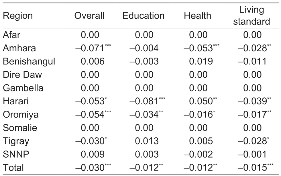
Table 7 Average treatment effect on the treated (ATT)decomposition by regions

There is one drawback of the PSM estimation,that it cannot provide consistent estimations of causal effects in the presence of a hidden bias. Thus,to check for the robustness of our PSM results and to control for an unobservable selection bias ESR is estimated. Before estimating ESR,the study checks whether the model is correctly identified or not in terms of the instruments used in the model. For the ESR model to be identified the issue of exclusion restrictions is an important criterion (Di Falcoet al.2011). A simple falsification test is employed following Di Falcoet al.(2011) and Shiferawet al.(2014)to test the validity of the instruments. The study employs the variables related to region-dummies (e.g.,Oromiya-Dummy and Harari-Dummy) as selection instruments in the outcome function and two other variables,crop rotation and access to credit services,after the falsification test (Appendix A).

The idea behind performing a falsification test is,“if a variable is a valid selection instrument,it will affect the adoption decision in the selection equation but it will not affect the outcome variable (aggregate deprivation score) among farm households that did not adopt the technology” (Di Falcoet al.2011). Appendix A shows that the variables Oromiya-Dummy,Harari-Dummy,crop rotation,and access to credit services can be considered as valid selection instruments as they are jointly statistically significant drivers of the decision to adopt or not adopt the technology under study as the bottom part of Appendix A shows (Model 1,χ2=114.42;P=0.00)but not for the aggregate deprivation score of the farm households that did not adopt the technology (Model 2,F-stat.=0.96,P=0.41).

In estimating the impact of the technology,we expect adoption to have MPI-reducing effects. However,adoption of CSAT by itself is potentially endogenous,which would lead to correlation between CSAT and the error term and biased estimates of coefficients.Endogeneity of adoption may arise from unobserved heterogeneity,reverse causality,or measurementerror. We control for endogeneity bias by estimating a simultaneous equations model with endogenous switching using the FIML approach. The FIML estimates of the ESR model are reported in Table 9. The second column gives the estimated coefficients of selection eq.(11) on adopting the specified technology whereas the third and fourth columns give the aggregate deprivation score estimated using eqs.(12a) and (12b) for the two farm household groups.10The ‘movestay’ command of Stata is used for estimating the endogenous switching regression model by FIML (Lokshin and Sajaia 2004).

Table 8 Degrees of overall deprivation and average treatment effect on the treated (ATT) by adoption status

The results of the ESR model shows that the estimated coefficient of correlation between the adoption (selection)equation and the aggregate deprivation score (outcome)equation (φj) is statistically significant. The results also show that both observed and unobserved factors influenced the decision to adopt CSAT and welfare outcomes given the adoption decision. The significance of the coefficient of correlation between the adoption equation and the welfare (aggregate deprivation score) of the adopters indicates that self-selection occurred in the adoption of improved agricultural technologies.

The differences in the aggregate deprivation score’s coefficients between farm households that adopted CSAT and those that did not show the presence of heterogeneity in the sample households (see Table 9,Columns 3 and 4).For example,the two groups (adopters and non-adopters)differ in factors like household age,Tigray-Dummy,extension service,family size,and marital status as the aggregate deprivation score equation of ESR shows. The aggregate deprivation score function of farm households that adopted improved agricultural technologies is significantly different from the aggregate deprivation score of farm households that did not adopt the technology and the likelihood-ratio test for joint independence of the three equations is reported in the last line of Table 9 and this is statistically significant.

In Column 2,Table 9 the selection equation shows that the decision to adopt the specified technology is determined by all factors except marital status,Tigray-Dummy,crop rotation,and household head’s sex.Household head’s age square and household size square negatively affected the technology adoption decision while the remaining significant variables are positively associated.

The results in Table 10 also show that using both ESR and PSM methods the impacts of the technology are largely consistent in the two methods such that CSAT leads to a reduction in the aggregate level of deprivation scores while findings are statistically significant.The findings also show that farm households that did not adopt the CSAT would have benefited significantly had they adopted it as indicated in the ESR results (ATU).

3.3.Mechanisms of poverty reduction pathways

The results in Tables 5 and 6 suggest that the effects of CSAT adoption on multidimensional poverty are largerthan the effects on consumption expenditure poverty. To explore the possible impact pathways,first we checked the correlation between consumption expenditure and deprivation score. The correlation between food consumption expenditures and total deprivation scores is negative (–0.199) and significant (P＜0.000). Similarly,the association between non-food consumption expenditures and total deprivation scores is also negative (–0.106) and significant (P＜0.001). Appendix H also shows a similar trend and confirms this fact.

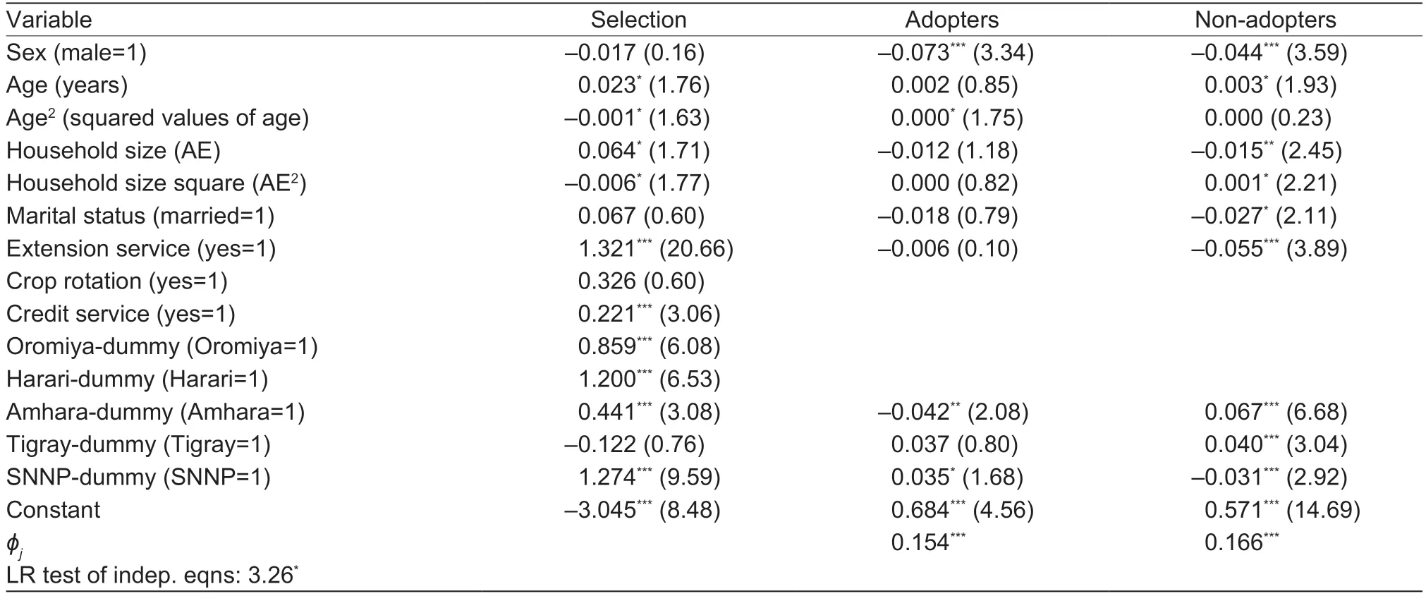
Table 9 Full information maximum likelihood (FIML) estimates of the switching regression model:Dependent variables:Adoption(1/0) and aggregate deprivation score (ci)

Again to assess the pathway empirically,we regressed total deprivation score on food and non-food consumption expenditure (in place of income due to lack of income data) following the approach proposed by Ogutu and Qaim (2019). The result shows that consumption expenditure gains contribute significantly to reducing MPI scores. Interestingly,the effect is stronger for nonfood expenditure than for food expenditure. Non-food expenditure leads to a 2.82% reduction in MPI scores while food expenditure contributes to a 2.51% fall in MPI scores. This result suggests that as CSAT adoption leads to a rise in incomeviaproduction (or productivity),the income gains are channeled to other non-food expenses including health,child education,contribution to community activities,and so on.

Thus,the results show that the possible impact pathway for the reduction in multidimensional due to the adoption of CSAT is through an increase in income/consumption expenditureviaimprovement in production gain. Alternatively,if farmers adopt CSAT,they are able to increase agricultural outputs through intensification or commercialization,which suggests that increase in crop production can generate the level of income required to make it a viable pathway from poverty or through an increase in consumption due to rise in income. Findings also state that at the micro-level there is evidence that crop production is a pathway from poverty (Harris and Orr 2014). This finding is similarly supported by previous works (e.g.,Amaduet al.2020) that finds CSAT is effective in resource poor and environmentally sensitive areas,and its adoption leads to a sustainable pathway to yield increases.

In the case of income rises; however,the question is whether the additional income is used for consumption expenditure or not. As stated above,the effects of CSAT on multidimensional poverty are primarily channeled through the income/expenditure pathway. This is confirmed in Table 11 below. As we may expect,results also show that CSAT adoption is positively correlated with total,food and non-food household expenditures (not reported here due to limited space).

Overall,these findings are consistent with some previous studies (e.g.,Hellin and Fisher 2018; Ogadaet al.2020),which demonstrate that CSAT and practices are feasible pathways out of poverty,especially when an intervention properly targets the relevant portion of the society. It is also possible to argue that in developing countries where most of the farming activities are dominated by smallholder farmers with small land holding and limited access to markets,returns from CSAT are larger. Targeting would be more effective if we know more about the technologies and improved targeting will ensure that CSAT makes a greater contribution to poverty reduction and ensuring food security as part of climate risk management.

Table 10 Endogenous switching regression model,expected conditional and average treatment effects of adoption on ci and a comparison with propensity score matching’s (PSM’s) results

4.Conclusion and policy recommendations

The study connects the multidimensional poverty methodology to the impact evaluation technique in the agriculture sector by using the PSM and ESR methods in combination with the Alkire and Foster counting approach for measuring MPI. This research contributes to the literature on the impacts of CSAT on multidimensional poverty in which previous studies less explored.Another novelty of the study is that it has introduced the mechanisms of poverty reduction pathway in which dominants of previous impact evaluation studies in agriculture neglected it.

In the unidimensional approach,the study uses consumption expenditure-based poverty measurement,and the results show that about 42% of the households are poor while the relative poverty measure reveals that about 47% of the households are poor. The results also indicate that adopters are slightly better-off than non-adopters implying that CSAT improves adopters’welfare. A comparison between sexes of household heads indicates that female-headed households are less impoverished as compared to male-headed households.A further regional disaggregation also shows that Benishangul is the most impoverished region (59.8%)followed by SNNP (57.1%).

Using MPI,about 59% of people are multidimensionally poor. The results concerning the impacts of CSAT on multidimensional poverty show that people are the most deprived in the education dimension (41.8%) followed by the standard of living dimension (34.6%),while indicatorwise,they are the most deprived in terms of years of schooling and while they are less deprived in access to clean water.

The empirical results also show that the adoption of technology reduces the overall deprivation in the range 2.0–3.0% while the living standards component drives the change in MPI indicating a reduction between 1.6–2.2%. Regionally the results also show the existence of difference in impacts of CSAT in which a high reduction in deprivation is observed in Amhara followed by the Oromiya region. The results also show that the impact is significantly higher among the severely deprived ones. The impact pathway analysis indicates that the reduction in multidimensional poverty due to the adoption of CSAT is through an increase in income/consumptionviaimprovement in production gain. An increment in crop production can generate the level of income required to make it a viable pathway from poverty or through an increase in consumption due to rise in income; where this channels more through the nonfood expenditure pathway. Finally,it was noted that the inclusion of additional dimensions of poverty improves its measurement. Thus,we conclude that CSAT is an important and effective mechanism towards achieving the Millennium Development Goal #1 and Sustainable Development Goals #1-2 and 12,13 and 15 in general.

The study has two major implications based on the findings. First,the results show that the extent of multidimensional poverty is very high,and the impact of technology varies across regions and by sex which requires concerted policy interventions. Policymakers should consider regional variations,community realities,and households’ characteristics to fight poverty and ensure other social welfare like food security,increase rural income,etc. At the country level,this may require a revision of the national poverty reduction strategies to incorporate the multidimensional aspects of deprivation and considering appropriate agricultural technologies that most affect multidimensional welfare indicators,especially poverty and its components in this case.

Second,the analysis also highlights that,though the level of income poverty seems lower,multidimensional poverty remains high which better indicates the status of households considered. In this regard,it is important to consider different climate-smart technology packages that are appropriate and relevant to location-specific cases,less time-consuming,and gender-neutral types of technologies. It is also indicated that CSAT is one of the best pathways to poverty reduction which implies that broader investment and scaling-up of adoption of various CSA packages is crucial. Future poverty alleviationpolicies and strategies should view poverty broadly and design appropriate multifaceted interventions.

Table 11 Mechanisms of poverty reduction pathway1)

Acknowledgements

The author is grateful to Professor Almas Heshmati(Jönköping International Business School (JIBS),Jönköping University,Sweden) for his meaningful support during writing of the research,editing and sending the paper for language edition and Professor Ashwini Phadnis(The Hindu Business Line,India) for the language edition service. The author also thanks the two referees for their meaningful comments on earlier versions of this paper.Thanks to Jönköping International Business School (JIBS),Sweden,for supporting the author to participate in various international conferences and workshops; invitation to JIBS,and many thanks to both Addis Ababa and Arsi Universities of Ethiopia,for the supports during the study.

Declaration of competing interest

The author declares that there is no conflict of interest.

Appendicesassociated with this paper are available on http://www.ChinaAgriSci.com/V2/En/appendix.htm