Coherent-driving-assisted quantum speedup in Markovian channels∗
2021-03-11XiangLu鹿翔YingJieZhang张英杰andYunJieXia夏云杰
Xiang Lu(鹿翔), Ying-Jie Zhang(张英杰), and Yun-Jie Xia(夏云杰)
Shandong Provincial Key Laboratory of Laser Polarization and Information Technology,Department of Physics,Qufu Normal University,Qufu 273165,China
Keywords: quantum dynamics control,quantum speed limit,Markovian dynamics
1. Introduction
Quantum speed limit time(QSLT)defined as the shortest time of evolution between two distinguishable states,[1–19]is a key method for characterizing the maximal evolution speed of a quantum system. The understanding of QSLT has been applied in quantum communication,[20,21]non-equilibrium thermodynamics,[22]quantum metrology,[23]quantum optimal control[24–27]and other fields. For a closed quantum system, the quantum speed limit usually has two different boundaries, namely Mandelstam–Tamm (M-T) bound[1]and Margolus–Levitin (M-L) type boundary.[2]However, in real situations,any quantum information process is inevitably subject to environmental noise. Hence, how to delimit QSLT in the nonunitary dynamics of the open system is followed up by more and more researchers in quantum information field. In Refs.[13,15],relative purity is used to define the QSLT of arbitrary initial state. Deffner and Lutz[28]unified the M-T and M-L boundaries of QSLT using the Bures angle for the open system. Then, in 2019, Campaioli et al. proposed a solution method of the QSLT of any quantum state in the process of unitary dynamics[28]and non-unitary dynamics.[29]Recently,a new bound of QSLT[30]for open systems was proposed using the gauge invariant and geometric natures of quantum mechanics.
Moreover, many valuable efforts have also been taken to exploration of QSLT in open systems under non-unitary evolution. For instance, the effects of entanglement on multipartite systems,[33–36]decoherence speed limit of the spin boson system,[37]the effect of coherent or excited state population on QSLT,[17,18,39,40]research on QSLT in non-equilibrium environment[41]and QSLT in classical and quantum systems.[42,43]In addition, Deffner and Lutz[14]firstly pointed out that the non-Markovian regime of the environment can promote the speedup of quantum process.Therefore, a common way to speedup the quantum evolution process is to transform Markovian dynamics into non-Markovian dynamics,[14–18,44–46]the corresponding scheme is also obtained in the experiment.[47]Even though the non-Markovianity of environment has been currently manipulated in few experiments, they are often limited to certain physical systems. Hence, how to look for an oversimplified way to design an operational and experimental implementation for quantum speedup without considering the non-Markovian dynamical behavior is necessary and extremely significant.
The Hamiltonian corrections through the action of coherent driving forces are often used to fight dissipative and decoherence mechanisms.[48–50]The coherent driving Hamiltonian corresponding to a simple quantum rotation operation on the qubit could be easily realized in a variety of actual physical systems.[51–54]Based on the effects of the coherent driving Hamiltonian, in this paper we calculate and analyze the dynamics of an open system in three typical decoherent noise channels(the phase-flip channel,the amplitude damping channel and the depolarizing channel). By choosing QSLT[29]as a description of the achievable evolution speed of the open system,it is interesting to show that,in the presence of the coherent driving,no-speedup evolution in the Markovian dynamics process can be transformed into quantum speedup evolution.We also analyze the best driving way to achieve the most degree of quantum speedup in the considered three noisy channels,respectively.Furthermore,it is worth mentioning that the dynamics of the system still retains Markovian behavior. That is to say, the coherent driving to the system can not transfer the original Markovian behavior to the non-Markovian behavior. Unlike the previous speedup scheme,this speedup scheme can be achieved in the Markovian regime, and does not have to generate the non-Markovian behavior of the dynamics.
The organization structure of this work is as follows. In Section 2,we introduce the calculation method of the dynamics of the system in detail. In Section 3, we mainly analyze the results of the quantum speedup of a qubit in three different noisy channels. In Section 4,we present the conclusion of this work.
2. Dynamics in Markovian channels
In order to get the density matrix at any time by a given initial state of a quantum system, we mainly discuss the one-qubit system under the classical noisy influence of environment. Now we introduce the Gorini–Kossakowski–Sudarshan–Lindblad(GKSL)master equation[58,59]

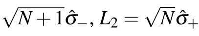
with
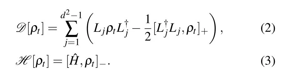
Equation(1)consists of two parts: the first is a purely dissipative term, and the second is a coherence-preserving contribution gauged by a Hamiltonian term. Here Ljare the Lindblad operators,γ is the damping parameter,and d is the dimension of the system. The symbols[···,···]±indicate the commutator (−) and anticommutator (+) brackets, respectively. The driving of Hamiltonian term in Eq.(1)can be expressed by

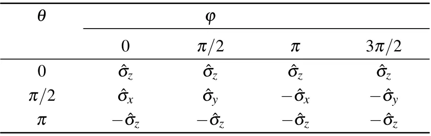
Table 1. Driving direction at different special angles.
In the operator basis (E00,E10,E01,E11) formed by the external products Eij=|i〉〈j|of the computational basis(here i,j=1,2), the Lindblad superoperator L[ρt] can be written as a 4×4 matrix. The evolutional density matrix of the qubit ρt=Φtρ0. Since γ in the Markovian channel does not involve time, the dynamic evolution operator Φtcan be acquired by Φt=Exp[tL],which can be expressed as
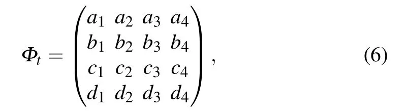
and then by rearranging the matrix Φtin terms of four bases,four 2×2 matrices(M1,M2,M3,M4)are expressed as
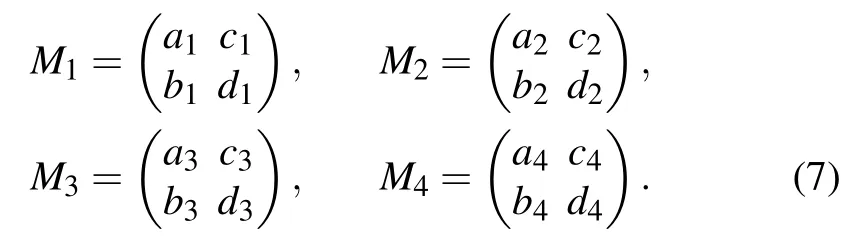

Then the reduced evolution density matrix ρtat any time can be expressed as

3. Quantum speedup of dynamics process
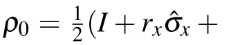
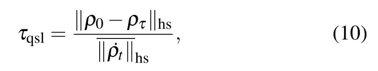
The coherent driving term acting on qubits can be easily implemented in experiments. As we all know,for the Markovian dynamics process,if no coherent driving term acts on the system (ω =0), the dynamics of quantum system would not be accelerated.[14,15]In order to illustrate the role of the coherent driving on the quantum speed of the open system,a proper QSLT could be effectually defined by the bound of minimal evolution time for arbitrary initial states ρ0to the corresponding target evolution state ρτ, facilitating to analyze the maximal evolution speed of an open system. In 2019, Campaioli et al. derived the expression of QSLT by relying on the Euclidean distance to measure the divisibility between two quantum states in a generalized Bloch sphere,[29]the QSLT has been defined as
3.1. Phase-flip channel
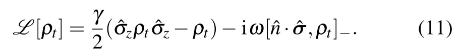
Phase-flip channel is a noisy process of pure quantum mechanics property. It describes the loss of quantum information without loss of energy, reflected in the decay of the off-diagonal elements of the density matrix with time. In this channel, the Lindblad operator is L1= ˆσz/2. Hence Eq. (1)can be rewritten as
Substituting operator basis (E00,E10,E01,E11) into Eq. (11)yields the matrix for each of the four bases,

Accordingly,we can obtain the Lindblad superoperator[49]of the phase-flip channel as follows:
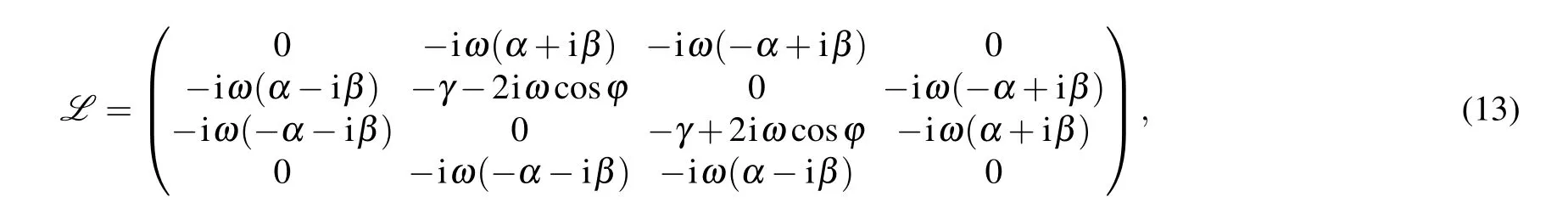
with α =sinθ cosϕ and β =sinθ sinϕ.
First, we analyze the effect of coherent driving term on the dynamics of the qubit in the phase-flip channel.Setting the initial state of the qubit in the maximal coherent state(rx=1,ry=rz=0),the quantum speed of this initial state cannot be accelerated in the Markovian phase-flip channel,as reported in Refs.[15,40]. Therefore,in the following,by inducing the coherent driving on the qubit and choosing certain driving direction angles,we would discuss the relationship between QSLT of the qubit and the driving parameter ω.
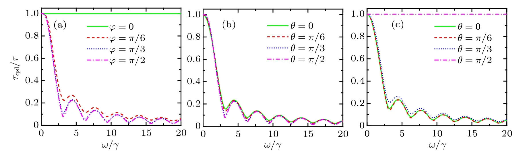
Fig.1. The relationship between QSLT and the driving strength ω in the phase-flip channel with γ =1: (a) driving the ˆσx–ˆσy direction,θ =π/2;(b)driving the ˆσz–ˆσy direction,ϕ =π/2;(c)driving the ˆσz–ˆσx direction,ϕ =0.
As shown in Fig.1,without coherent driving(ω=0),the whole quantum process cannot be speedup, i.e., τqsl/τ =1.While for the case ω /=0 (adding the external coherent driving on the qubit),the values of τqsl/τ <1 have been obtained.In addition, the oscillation reduction behavior of τqsl/τ will appear with increasing the driving strength ω. This means that the original no-speedup dynamics process has become the speedup dynamics process by introducing an external coherent driving operating on the qubit in the phase-flip channel.Moreover, from Fig.1, we also find that, with the increasing ω/γ,QSLT could tend to zero numerically. Here, we must remind the fact that τqsl/τ →0 is physically meaningless.At this time,τqsl/τ →0 corresponds to a very loose bound of the quantum speed limit,and it can not mean the infinite acceleration of the evolution of the system.

Combining Fig.2 with Table 1, it can be seen that no matter how strong the driving is, only the driving in the ˆσxdirection has no-speedup effect on the whole quantum process, i.e. τqsl/τ =1. Therefore, it can be considered that for this channel, the driving ˆσxdirection does not contribute to quantum speedup. For the coherent driving in any other directions,the quantum process can be speedup to different degrees,i.e.,τqsl/τ <1. Furthermore,a speedup evolution of the open system would be preferable to deal with the robustness of quantum simulators and computers against decoherence. How to explore the maximum speedup condition of quantum process is meaningful. Therefore, the minimum value of τqsl/τ must be found to characterize the maximum speed of evolution. However, according to the different driving strengths,the driving direction angles (θ and ϕ) corresponding to the minimum QSLT are also different. For example in Fig.2(a)in a quarter of one period (0 to π/2), when the two driving angles θ =0 and ϕ =0,the QSLT takes the minimum value,that is, at this time the dynamics of the qubit can be speedup most. In Fig.2(b) the minimum value of QSLT will appear when θ =0.14π and ϕ =0.035π. As ω increases,this condition is going to θ =π/2 and ϕ =π/2 in Figs.2(c)and 2(d).Therefore,with the increase of driving strength ω,the optimal driving operating changes from ˆσzdirection to ˆσydirection.In order to find the driving direction with the best speedup effect of this channel, the value of its driving parameters must be considered. For the smaller driving strength, the optimal driving direction is obtained near the ˆσzdirection. While for the larger driving strength,the optimal driving direction is obtained near the ˆσydirection.
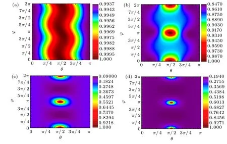
Fig.2. The relationship between QSLT and driving angles of the coherent driving in the phase-flip channel with τ =1: (a) ω/γ =0.2, (b)ω/γ =1,(c)ω/γ =3,(d)ω/γ =5.
3.2. Amplitude damping channel
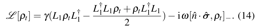
Similar to the previous method,by substituting operator basis(E00,E10,E01,E11)into Eq.(14)to get the matrix for each of the four bases,the Lindblad superoperator[49]of the amplitude damping channel is as follows:
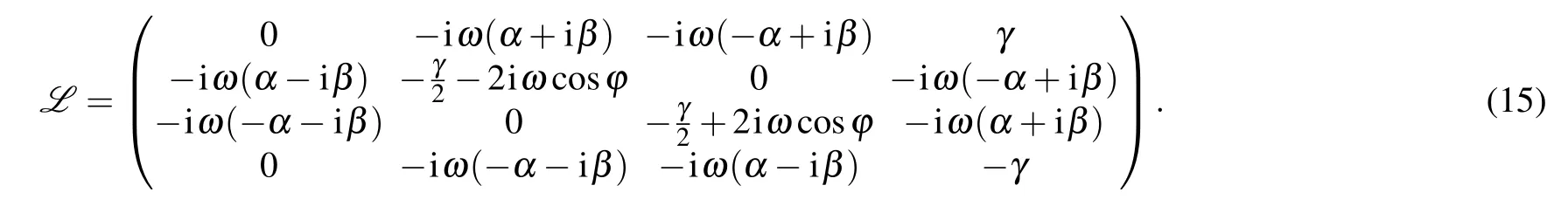
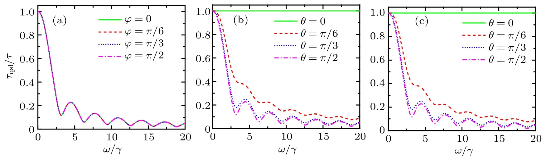
Fig.3. The relationship between QSLT and driving strength ω for the qubit in the amplitude damping channel with τ =1,N=0: (a)driving the direction,θ =π/2,(b)driving thedirection,ϕ =π/2,(c)driving the direction,ϕ =0.
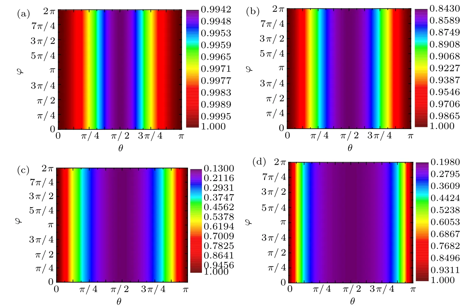
Fig.4. The relationship between QSLT and driving angles of the coherent driving in the amplitude damping channel with τ =1,N =0: (a)ω/γ =0.2,(b)ω/γ =1,(c)ω/γ =3,(d)ω/γ =5.

3.3. Depolarizing channel

The Lindblad superoperator[49]in the depolarizing channel is as follows:
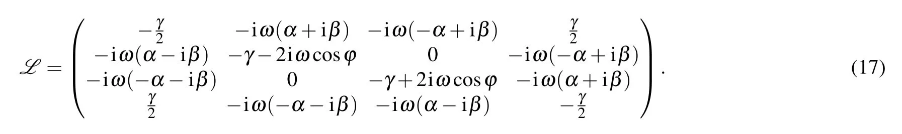
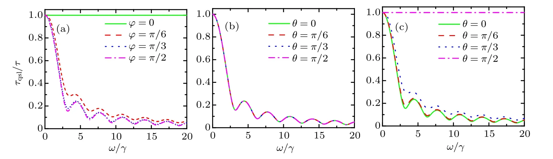
Fig.5. The relationship between QSLT and the driving strength ω for the qubit in the depolarizing channel with γ =1: (a)driving the ˆσx–ˆσy direction,θ =π/2,(b)driving thedirection,ϕ =π/2,(c)driving thedirection,ϕ =0.


Fig.6. The relationship between QSLT and driving angles of the coherent driving in the depolarizing channel with τ =1: (a)ω/γ =0.2,(b)ω/γ =1,(c)ω/γ =3,(d)ω/γ =5.
3.4. Physical reason for speedup
In the above subsections,we mainly discuss the quantum speedup under the coherent Hamiltonian driving in three different Markovian channels. As we all know,quantum speedup evolution of an open system is usually induced by the non-Markovianity[55–57]of the environment. However,for the evolution of this model under the Lindblad main equation described by Eq.(1),no matter how the driving term is adjusted,the dynamics of the system cannot exhibit the transition from Markovian behavior to non-Markovian behavior. To prove it,we have used the Breuer–Laine–Piilo method[57]to calculate the non-Markovianity of the above three channels. We confirm that the dynamics of the system still maintains the Markovian property under the coherent driving. Interestingly,unlike other speedup models mentioned previously,[14,18,39,45,46]this speedup scheme in our work can be achieved in the Markovian regime,and does not have to be generated the non-Markovian behavior of the dynamcis.
In Ref.[29],the authors described the geometric distance as the numerator of state space by generalized Bloch vectors.This geometric distance D(ρ,σ)=‖r −s‖hsis also defined as the numerator of τqsl. That connects r =ρ0, s=ρτ. To further make the analysis of the intrinsic physical reason for quantum speedup induced by the coherent driving operation on the system, we concern the geometric distance D(ρ0,ρτ),which can be written as D(ρ0,ρτ)=‖ρ0−ρτ‖hs.We compare τqsl/τ and D(ρ0,ρτ)in the above three different channels. In the Fig.7,we take three different sets of driving direction angles for the above three channels. For the green solid line in Fig.7,we choose the driving direction angles that cannot lead to speedup in each channel, i.e., τqsl/τ =1. The geometric distance D(ρ0,ρτ) is going to increase smoothly and monotonically. While for the red dashed line in Fig.7, we choose the driving angles that can acquire the maximum accelerated evolution of the dynamics process,i.e.,τqsl/τ is the minimum.The geometric distance D(ρ0,ρτ)increases in oscillating with the actual evolution time τ. For the blue dash-dotted line,we take an arbitrary set of angles for comparison.We can find that the geometric distance D(ρ0,ρτ)is also oscillating up.
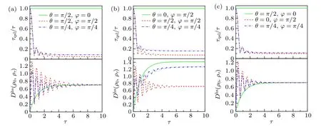
Fig.7. The QSLT τqsl/τ and the geometric distance D(ρ0,ρτ)of the dynamics evolution from the initial state to the final state as a function of the actual evolution time τ,with ω/γ =5: (a)the phase-flip channel,(b)the amplitude damping channel,(c)the depolarizing channel.
This phenomenon shows that for a speedup quantum process, the geometric distance between the initial state and the target final state would oscillate with the actual evolution time.Especially, the larger the oscillation, the smaller the QSLT of the quantum process, indicating that the system can be speedup more. Similarly, we can find that with the increase of the actual evolution time τ, both τqsl/τ and the geometric distance D(ρ0,ρτ) tend to the stable value. The reason is that,when the actual evolution time increases to a certain extent, the density matrix of the qubit hardly changes, and the decoherence process has been completed. Consequently, it is worth noting that the coherent driving term added to the open system does not lead to the non-Markovian behavior. However, the coherent driving parameters could cause the oscillation changes of the geometric distance D(ρ0,ρτ) between the initial state ρ0and the target final state ρτ. Somewhat contrary to the previous speedup scenarios by the controllable non-Markovianity,our results clearly show that the oscillation changes of the geometric distance D(ρ0,ρτ)caused by the coherent driving are the intrinsic physical reason for quantum speedup in our scheme.
4. Conclusion
As we all know,the quantum evolution speed of an open system can never be accelerated in the Markovian regime without any operators on the system. One unitary coherent driving Hamiltonian corresponding to a simple quantum rotation operation on the qubit can be easily accomplished in a variety of actual physical systems in experiments,so in this work we mainly demonstrate that a speedup evolution of the system could be implemented by the action of the coherent driving on the system in the phase-flip channel, the amplitude damping channel and the depolarizing channel.

杂志排行
Chinese Physics B的其它文章
- Novel traveling wave solutions and stability analysis of perturbed Kaup–Newell Schr¨odinger dynamical model and its applications∗
- A local refinement purely meshless scheme for time fractional nonlinear Schr¨odinger equation in irregular geometry region∗
- Quantifying entanglement in terms of an operational way∗
- Tunable ponderomotive squeezing in an optomechanical system with two coupled resonators∗
- State transfer on two-fold Cayley trees via quantum walks∗
- A concise review of Rydberg atom based quantum computation and quantum simulation∗