A meshless algorithm with the improved moving least square approximation for nonlinear improved Boussinesq equation*
2021-01-21YuTan谭渝andXiaoLinLi李小林
Yu Tan(谭渝) and Xiao-Lin Li(李小林)
School of Mathematical Sciences,Chongqing Normal University,Chongqing 400047,China
Keywords: meshless,improved moving least square approximation,nonlinear improved Boussinesq equation,convergence and stability
1. Introduction
The nonlinear improved Boussinesq equation[1]is a new form of the famous Boussinesq equation.[2,3]By using uxxttinstead of uxxxx, the improved Boussinesq equation is physically stable and thus effectively overcomes the unrealistic instability of the bad Boussinesq equation. The improved Boussinesq equation can be used to model some physical phenomena such as sound waves,[1]acoustic waves on elastic rods,[4]and plasma waves at right angles to the magnetic field.[5]Over the past four decades, some numerical methods, such as the finite difference method (FDM),[6–9]the finite element method (FEM),[6,10]the finite volume element method(FVEM),[11,12]the Fourier pseudospectral method,[13]the radial basis functions method,[14]the local discontinuous Galerkin (LDG) method,[15]and the multisymplectic method,[16]have been adopted to obtain approximate solutions of the improved Boussinesq equation.
Meshless methods[17]have been rapidly developed in the past thirty years to mitigate the meshing-related issues in classical numerical methods such as the FDM and the FEM.Apart from the absence of elements,another outstanding merit of meshless methods is that, meshless shape functions and then meshless solutions are frequently generated with high accuracy. The moving least square (MLS) approximation is one of the most crucial approach to generate meshless shape functions.[17–21]Some improvements of the MLS,such as the interpolating MLS,[22,23]the complex variable MLS,[24–26]the improved complex variable MLS,[27]the improved interpolating MLS,[28]the complex variable interpolating MLS,[29]the stabilized MLS,[30]and the augmented MLS,[31]have also been proposed to enhance the performance of the MLS.
The improved moving least square (IMLS)approximation[32]is an improved version of the MLS approximation. By using weighted orthogonal basis functions instead of polynomial basis functions, the IMLS produces diagonal system matrices and then possesses a higher computational efficiency than the MLS.Recently,shifted and scaled basis functions have been used to improve the computational stability and precision of the IMLS approximation.[33]Based on the IMLS approximation, meshless methods such as the boundary element-free method,[17,32]the improved elementfree Galerkin method,[17,34–36]and the improved Galerkin boundary node method[37]have been proposed and implemented for problems in various fields of physics and engineering.
In this paper,an IMLS meshless method is developed for the numerical solution of the nonlinear improved Boussinesq equation. After the approximation of temporal derivatives,the original time-dependent improved Boussinesq equation is reduced to a set of time-independent equations. Then,the IMLS approximation is used to establish the systems of discrete algebraic equations,where shifted and scaled basis functions are used to guarantee convergence and stability of numerical results. Finally, an iterative algorithm is presented to solve the nonlinear algebraic systems. Numerical experiments involving propagation of single solitary wave and collision of two solitary waves are presented to demonstrate the efficiency of the method. Numerical results reveal that the current IMLS meshless method yields much less error than the FDM, the FEM,the FVEM and the LDG method.
2. Problem description
Consider the following nonlinear improved Boussinesq equation:
3. Approximation of temporal derivatives
According to the Taylor series, the temporal derivatives can be approximated by the difference quotient as[32]
4. Discretization of spatial derivatives
In the IMLS approximation, the solutions uk+1(x) of Eqs.(7)and(10)can be approximated as
5. Algorithms
In view of Eq. (19), the algebraic systems given in Eq. (18) are nonlinear. The following iterative algorithm is adopted to solve these nonlinear systems.
Algorithm 1 Set l =0 and uk+1,l=uk, and choose a tolerance ε >0.
Theorem 1 Let


6. Numerical results
6.1. Propagation of single solitary wave
Consider the improved Boussinesq equation(1)with the initial conditions

The propagation of the single solitary wave and the associated error |u-uh| for x ∈[-80,140] and t ∈[0,72] are presented in Fig.1,while the results at t=72 are presented in Fig. 2. In this analysis, we use the time-step size τ =0.001,the nodal spacing h=0.1, and various amplitudes A=0.25,0.5, 0.75, and 0.9. It can be observed from these figures that the single solitary wave propagates with no change in form,and the current IMLS method obtains very accurate numerical results.
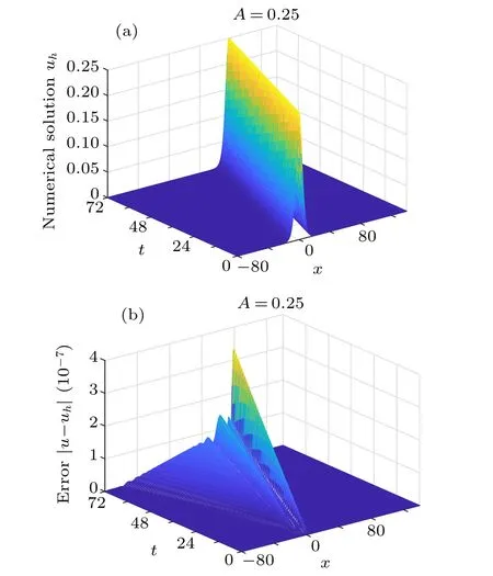
Fig. 1. Results of (a) the numerical solution and (b) the associated error obtained using h=0.1 and τ =0.001 for x ∈[-80,140]and t ∈[0,72].
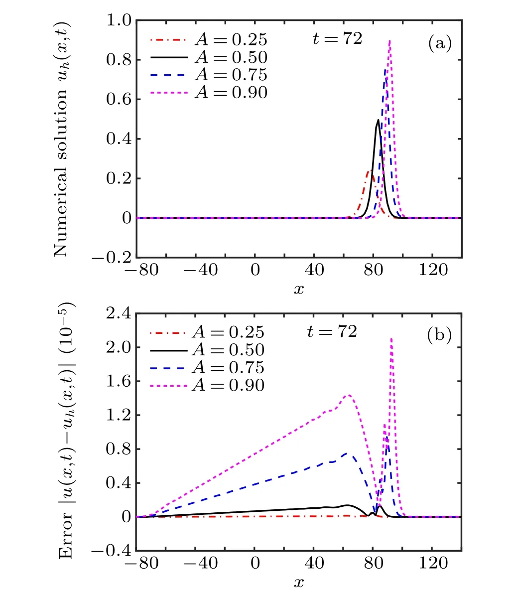
Fig.2. Results of(a)the numerical solution uh and(b)the associated error|u-uh|obtained using h=0.1 and τ =0.001 at t=72.
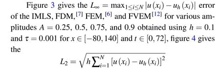
and L∞errors of the IMLS and LDG[15]for A = 0.5, x ∈[-100,100],and t ∈[0,1],while figure 5 gives the L2and L∞errors of the IMLS,FVEM1,[11]and FVEM2[12]for A=0.5,x ∈[-60,100], and t ∈[0,1]. It can be found from Figs.3–5 that the current IMLS method produces much less error than the other methods.
Fig. 3. Comparison of the L∞error for FDM,[7] FEM,[6] FVEM,[12] and IMLS.

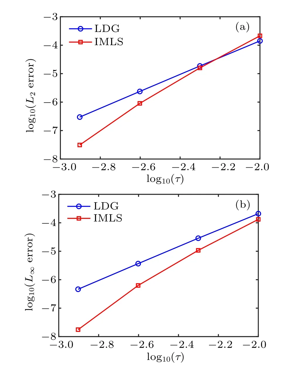
Fig. 4. The comparison of (a) L2 and (b) L∞errors for the LDG[15] and IMLS.

Fig. 5. The comparison of (a) L2 and (b) L∞errors for FVEM1,[11]FVEM2,[12] and IMLS.
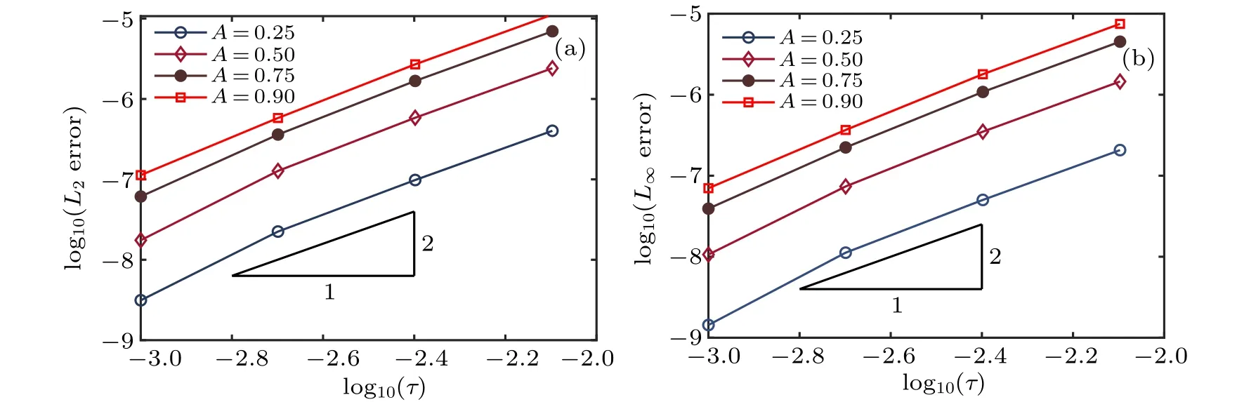
Fig.6. Convergence of the IMLS method with respect to the time-step size τ obtained using h=0.1: (a)L2 and(b)L∞errors.
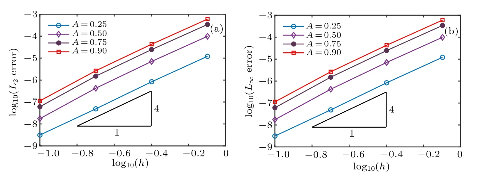
Fig.7. Convergence of the IMLS method with respect to the nodal spacing h obtained using τ =0.001: (a)L2 and(b)L∞errors.
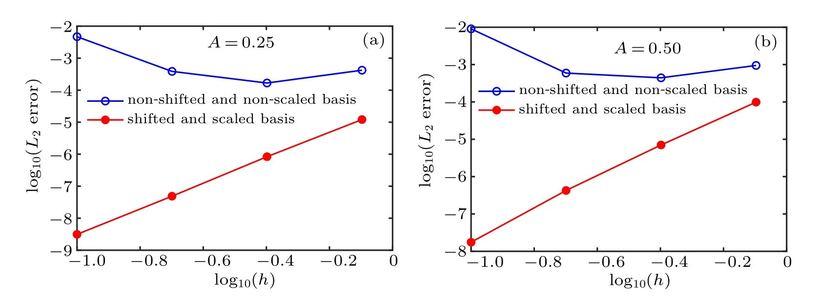
Fig.8. Convergence and stability of the IMLS method using two kinds of basis functions.
In the original IMLS method, the non-shifted and nonscaled basis functions given in Eq.(15)are used to form shape functions. While in the current IMLS method,the shifted and scaled basis functions given in Eq.(16)are used to form shape functions. Convergence and stability of the IMLS method based on the two kinds of basis functions are shown in Fig.8.In this analysis, we use x ∈[-60,100], t ∈[0,1], τ =0.001,and A=0.25 and 0.5. It can be found that the numerical results obtained by the non-shifted and non-scaled basis are instability and not convergent,while the results obtained by the shifted and scaled basis converge rapidly and monotonously.Therefore, the shifted and scaled basis produces lower computational error and has better numerical convergence and stability than the non-shifted and non-scaled basis.
6.2. Collision of two solitary waves
Consider the improved Boussinesq equation(1)with the initial conditions
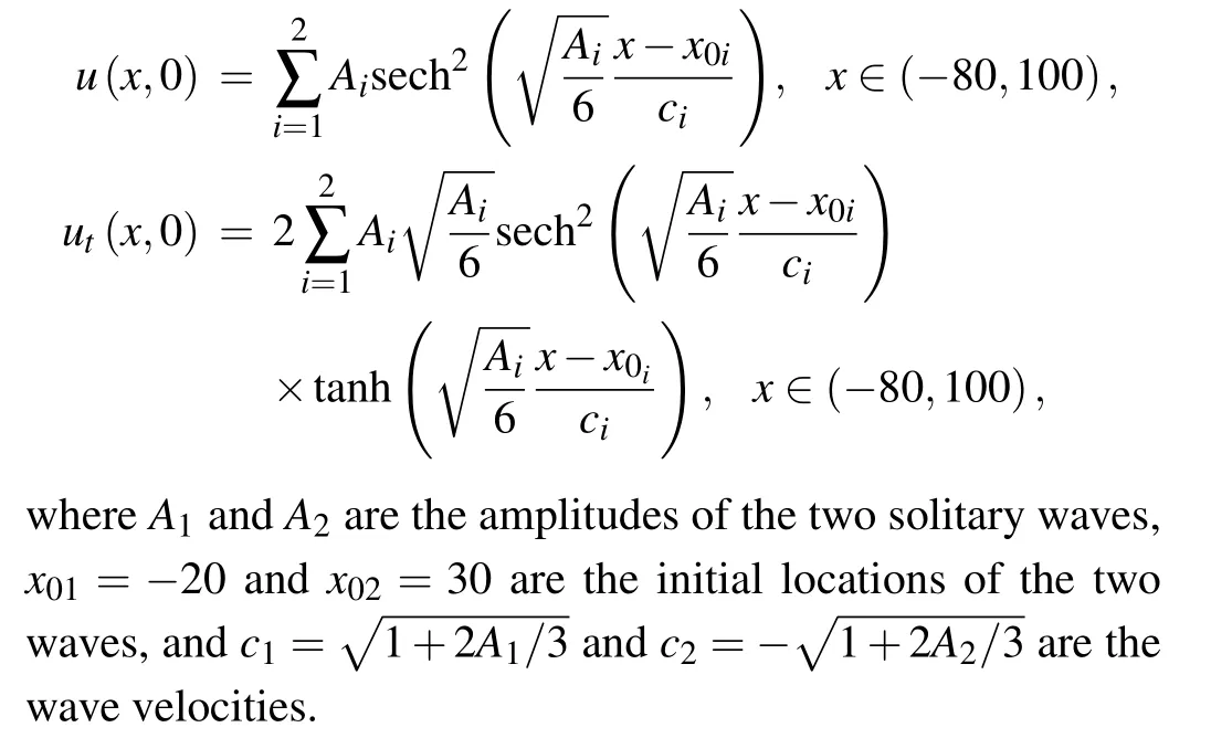
Figure 9 gives the evolution of the two solitary waves for equal amplitudes A1=A2=0.4 and A1=A2=2.0, figure 10 gives the evolution for unequal amplitudes A1=0.4 and A2=0.5,1.5 and 2.5,while figure 11 gives the numerical solutions for various amplitudes at t=60. In this analysis,we use the time-step size τ=0.001 and the nodal spacing h=0.1.
We can see from Figs.9 and 10 that the two waves begin to move independently,then collide gradually,and finally pass through each other. At the collision time, the two waves almost disappear,but after a while,they appear and regain their amplitudes, shapes and speeds. Besides, figures 9(a), 10(a),and 11(a) show that there are invisible secondary waves after the collision and thus the collision is elastic in the case of A1=A2=0.4,and the case of A1=0.4 and A2=0.5. However, figures 9(b), 10(b), 10(c), and 11(b)show that there are visible secondary waves after the collision and thus the collision is inelastic in the case of A1=A2=2.0, and the two cases of A1=0.4 and A2=1.5 and 2.5. Moreover,the larger amplitudes are, the stronger secondary waves are. Thus, the collision and the inelasticity rely on the amplitudes of the two solitary waves.
These results are in good agreement with those obtained by FDM,[7–9]FEM,[10]FVEM,[11,12]Fourier pseudospectral method,[13]radial basis functions method,[14]and LDG method.[15]
To show the collision quantitatively, Table 1 gives the values of the inelasticity coefficient K=Am/max(A1,A2)obtained by the current IMLS method, FDM,[7]FVEM,[12]and LDG.[15]Here,Amis the maximum joint amplitude at the collision time. It can be found that the IMLS values are similar as those in Refs.[7,12,15].
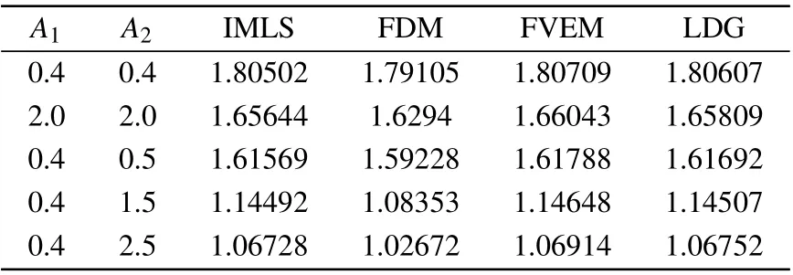
Table 1. The inelasticity coefficient K for various amplitudes.
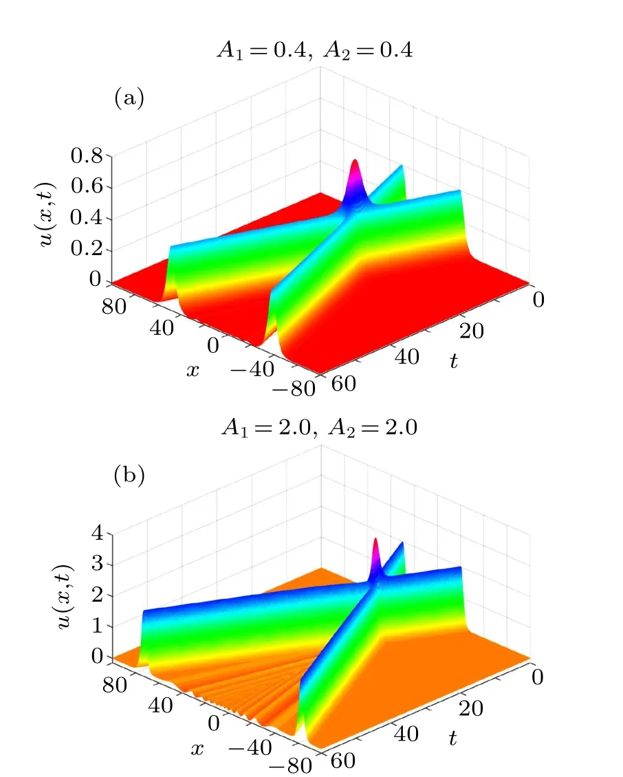
Fig. 9. Collision of two solitary waves for (a) A1 = A2 = 0.4 and (b)A1=A2=2.0.
Fig.10. Collision of two solitary waves for(a)A1=0.4 and A2=0.5,(b)A1=0.4 and A2=1.5,and(c)A1=0.4 and A2=2.5.
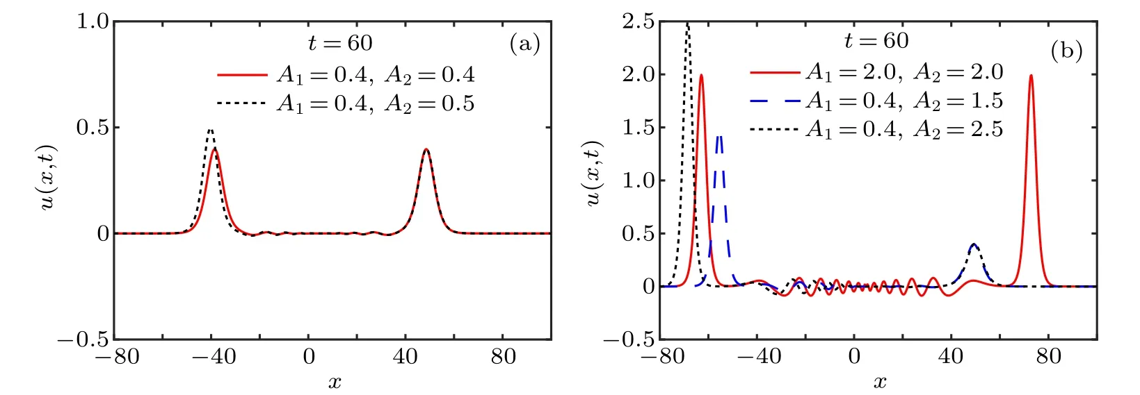
Fig.11. Results of the solutions for various amplitudes at t=60.
7. Conclusions
An IMLS meshless method is developed in this paper for the numerical analysis of the nonlinear improved Boussinesq equation. To illustrate the accuracy, convergence and efficiency of the method,numerical experiments involving propagation of single solitary wave and collision of two solitary waves are presented. Computational errors are compared with those obtained by FDM, FEM, FVEM, and LDG methods.These comparisons reveal that the current IMLS method yields much less errors. Besides, numerical results indicate that the errors of the IMLS method decrease rapidly as the time-step size and the nodal spacing decrease, and the method owns very good convergence properties with the second-order accuracy in time and the fourth-order accuracy in space. Moreover,the shifted and scaled basis functions produce lower error and have better numerical convergence and stability than the previously non-shifted and non-scaled basis functions. Future investigations can consider the performance of IMLS method for other nonlinear partial differential equations such as the unsteady Schr¨odinger equation,[35]Camassa and Holm equation,[36]Kadomtsev–Petviashvili equation,[39]and Euler equation.[40]
杂志排行

Chinese Physics B的其它文章
- Numerical simulation on ionic wind in circular channels*
- Interaction properties of solitons for a couple of nonlinear evolution equations
- Enhancement of multiatom non-classical correlations and quantum state transfer in atom–cavity–fiber system*
- Protein–protein docking with interface residue restraints*
- Effect of interaction between loop bases and ions on stability of G-quadruplex DNA*
- Retrieval of multiple scattering contrast from x-ray analyzer-based imaging*