A Combined Alignment Method for Strapdown Inertial Navigation System on Stationary Base

Shuai Chen, Xinzhi Liu, Qian Sun and Ya Zhang

(1.School of Information and Control Engineering, Liaoning Shihua University, Fushun 113001, Liaoning, China;2. Department of Applied Mathematics, University of Waterloo, Waterloo N2L3G1, Canada;3. College of Information and Communication Engineering, Harbin Engineering University, Harbin 150001, China;4. School of Electrical Engineering & Automation, Harbin Institute of Technology, Harbin 150001, China)

Abstract: Owing to the weak observability of the azimuth misalignment angle, alignment accuracy and time are always the contradictory issues in the initial alignment process of Strapdown Inertial Navigation System (SINS), which requires a compromise between them. In this paper, a combined alignment mechanism is proposed to construct an observable and controllable system model, which can effectively achieve higher azimuth alignment accuracy during the fixed time period. First, the Reduced Order Kalman Filter (ROKF) alignment algorithm was utilized to calculate the misalignment angles in parallel with the classical gyrocompass alignment algorithm. Then, the misalignment angles calculated by the gyrocompass alignment method were used to formulate the augmented measurement model with zero velocity models. Finally, the zero velocity model of the ROKF method was switched into the augmented measurement model when the azimuth misalignment angle of the gyrocompass alignment method was close to steady situation. The combined alignment method was analyzed reasonably by the observability and the mathematical deduction. The comparison results of the numerical simulation and the experimental data test showed that the combined method had good performance in terms of estimation accuracy and consistency of the alignment results.

Keywords: inertial navigation; instrumentation and measurement; gyroscopes; accelerometers; Kalman filter; measurement errors

1 Introduction

Strapdown Inertial Navigation System (SINS) is widely used in vehicles, ships, aviation, aerospace, and other fields due to the characteristics of autonomy, concealment, strong anti-interference ability, and comprehensive navigation information[1]. As a critical step of SINS, initial alignment technique is mainly used to determine the precise Direction Cosine Matrix (DCM). Then SINS completes the subsequent navigation solution process through the DCM. In the initial alignment process, alignment time and accuracy are often used to measure the quality of the initial alignment process, but the relationship between them is often contradictory. Therefore, many researchers have conducted in-depth studies to try to change this situation.

The reason for the contradiction between alignment time and accuracy is that the convergence of azimuth misalignment angle takes a long time. To solve this problem, the estimation of the horizontal attitude misalignment angle was used to calculate the azimuth misalignment angle[2], so as to realize the fast initial alignment process of SINS on stationary base. Since the theoretical estimation error of azimuth misalignment angle is mainly caused by the east gyro drift, an east gyro drift model was established to heighten the observability of the system and improve the alignment accuracy of the azimuth misalignment angle[3]. Unfortunately, low-pass filters need to be designed and used separately in the above two methods, and the alignment results of azimuth misalignment are very sensitive to the noise of inertial devices[4]. Since drift and unknown noise characteristics of inertial devices are the real causes of misalignment angle errors, some adaptive filter algorithms have been proposed to solve unknown noise problems and system stability problems, such as Adaptive Kalman Filter[5], Sage-Husa adaptive Kalman filter[6], Bilinear Recursive Least Square based on nonlinear adaptive filter[7], Adaptive Kalman Filter based on measurement residual[8], Adaptive Cubature Kalman Filter[9], and Adaptive Unscented Kalman Filter[10]. However, Kalman filter (KF) is always an optimal alignment method for the initial alignment of stationary base when the noise characteristics of inertial devices satisfy the Gaussian noise distribution[8].

In the case of known inertial sensor drift, the theoretical misalignment angle error can be easily obtained by the error analysis of SINS equations. It is well known that the main factor affecting the misalignment angle estimation is the constant biases and drifts of inertial sensors[8]. If the drifts and biases of the inertial sensors can be carried out, the misalignment angle errors can be easily driven to near zero. Although some methods can improve the alignment accuracy or the inertial sensor errors by the utilization of the translocation agency or turntable[11-12], they will introduce a new uncompensated error, and the designed extra devices can increase the complexity of the system and reduce the system reliability[12-13].

Any other method that formulates the error models of the sensors as the augmented measurement models[4,14-15]can increase the observability of the azimuth misalignment angle. As the component of earth rotation is included in the output of the gyroscope under the environment of stationary base, the method[4]that employs the whole east gyro output as the augmented measurement state is inexplicable. Some augmented measurement methods with sensor errors are reasonable to improve the alignment accuracy and the convergence speed of the initial alignment process for SINS[14-15]. With the observability analysis of the revised model, some observability degrees of the state variables are improved by the introduction of the sensor error model. However, the rank of the observability matrix has no change or the change of the observability degree because the azimuth misalignment angle is not clear.

Gyrocompass alignment method is also an effective way to realize alignment process, which depends on the design of control parameter and alignment time. In order to shorten the alignment time, a new method named forward and backward processes for INS alignment was proposed based on the full use of sensor data[16-17], in which the inertial sensor data is saved by the navigation computer and repeatedly used in both forward and backward sequences. The convergence time can be compressed by using this approach, while the theoretical alignment errors which are influenced by the inertial sensor errors cannot be minified.

For the purpose of decreasing the theoretical error that exists in the estimated results of the misalignment angle, a combined alignment mechanism is proposed in this paper to refine the estimation accuracy of the azimuth misalignment angle. From the perspective of improving the observability degrees of the system states, a fully controllable and observable system model was constructed by the method of the combined alignment. First of all, the Reduced Order Kalman Filter (ROKF)[18]was used in the initial alignment process before the combination stage, which only have five dimensional vectors and two dimensional measurement vectors. Meanwhile, the most commonly used gyrocompass alignment method was adopted in the whole initial alignment process. The compensated DCM, which is the DCM in the gyrocompass alignment method, was utilized to calculate the misalignment angles with the uncompensated DCM from the ROKF method. When the estimated results from both methods were close to convergence, the calculated misalignment angles would be augmented to the measurement model, and then the combined alignment process was started based on this augmented model. The whole process for the combined alignment mechanism can be implemented by the above scheme. Since the compensated DCM contains the attitude angle, theoretical estimation error, and calculation error, and the uncompensated DCM consists of the attitude angle, estimating misalignment angle, theoretical estimation error, and calculation error, rough misalignment angles can be achieved by the matrix operation. Through the analysis of the observability and the mathematical deduction, the combined method had higher estimation accuracy than that of the conventional alignment method. Although there was no compensation for sensor drift, the estimation accuracy of the misalignment angle was improved. The numerical simulation results and the experimental data test verified the correctness and practicability of the combined method.

The remainder of this paper is organized as follows. In Section 2, the error propagation models for the ROKF alignment method and the gyrocompass alignment model are introduced. In Section 3, the combined alignment mechanism is performed based on the error propagation model, and then the rationality of the combined method is analyzed by the observability analysis and the mathematical deduction. Section 4 presents the result of numerical simulation along with the specific statistical analysis. To verify the effectiveness and practicability of the combined alignment method, the data acquisition experiments are designed and the actual alignment results are analyzed in Section 5. Finally, conclusions are drawn in Section 6.

2 Error Model of Initial Alignment for SINS

Owing to the development of the coarse alignment method based on the inertial frame for SINS, the error propagation model of small misalignment angle is most likely to be applied to practical applications[3,19-21]. Because the misalignment angle is small, the initial alignment model can be approximated as a linear model, but the azimuth misalignment error cannot be neglected in navigation calculation compared with the horizontal attitude misalignment errors. Therefore, the linear error model based on KF is chosen as the initial alignment model in this paper.

2.1 Error Propagation Model for ROKF Alignment Method

The navigation frame (n-frame) in this paper is the local East-North-Up frame[22]. In then-frame, the error equations of misalignment angle and velocity error can be written as

For the transportation on the ground, the vertical channel can be ignored because of the application environment. Without the vertical velocity, the attitude errors and velocity errors equations can be expressed as

(1)

(2)

where the subscriptsE,N, andUdenote the three axis along then-frame; andR,L, andgrepresent the radius of earth, local latitude, and the local gravity, respectively.

In general, the inertial sensor constant errors are considered as the state variables, due to the navigation accuracy affected by the constant errors. To facilitate the proposed combined mechanism in Section 3, the ROKF alignment model was built in this section. The misalignment angles and velocity errors were selected as state variables as

(3)

whereX=[δVEδVNφEφNφU]T,

andW=[wAEwANwGEwGNwGU]T, whereWdenotes the process noise which satisfies the Gaussian distribution, andwAE,wAN,wGE,wGN, andwGUare the random biases of the accelerometers and random drifts of the gyroscopes, respectively.

The zero velocity model used in this section is as follows:

Z=HX+V,V∶N(0，R)

(4)

whereZ=[δVEδVN]T,V=[vEvN]T,Vis the measurement noise variable which satisfies the Gaussian distribution,vEandvNare the random errors of velocity error variables, andH=[I2×202×3].

2.2 Gyrocompass Alignment Model

(5)

(6)

On the stationary base, as the true velocity of the carrier was equal to zero, which was the same as the KF alignment model, the velocity and attitude error models were also the same as those in Eqs.(1)-(2). However, in the gyrocompass alignment method, the symbol before the gyroscope error items was exactly opposite with that in Eq.(2). The level alignment is based on the second order horizontal loop, and the azimuth alignment employs the third order gyrocompass alignment loop, which is based on the two horizontal loops in the north. Figs.1-2 show the schematic diagram of the gyrocompass alignment.

In Fig.2, the variableK(s) is commonly selected as

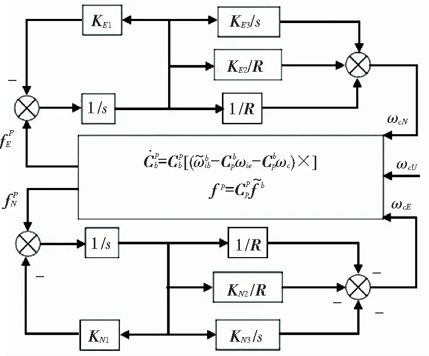
Fig.1 Schematic diagram of gyrocompass alignment in leveling loop

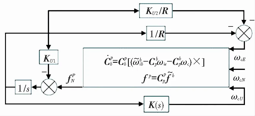
Fig.2 Schematic diagram of gyrocompass azimuth alignment

VariablesKEi,KNi, andKUj(i=1, 2, 3;j=1, 2, 3, 4) are the control parameters which can be calculated by the following equations:

KE1=KN1=3σ

3 Design of the Combined Alignment Method for SINS

3.1 Scheme of the Combined Alignment Method

According to the error analysis in Refs.[22-25], it is known that the gyrocompass alignment method nearly has the same alignment accuracy as the KF alignment method in the case of constant inertial sensor errors, but the symbols of the horizontal misalignment angles are opposite.

(7)

(8)

whereδφdenotes the theoretical estimation error of the misalignment angle. The overbar in Eq.(7) and the double overbar in Eq.(8) represent the steady errors of the KF alignment and the gyrocompass alignment, respectively.

For the initial alignment process of SINS, the constant drift of the inertial sensor is not estimable, so the theoretical error of the misalignment angle occurs in Eqs.(7) and (8). Although researchers have conducted a large amount of research on sensor error compensation, all the proposed methods need to compensate the inertial sensor error with the extra mechanical equipment. To avoid the increase of system complexity and the occurrence of additional errors caused by auxiliary equipment such as rotating modulation technology, a combined alignment mechanism is proposed in this section. When the azimuth alignment results of the two alignment methods enter the azimuth stabilization stage, the measurement model is switched to the measurement augmented model to realize the combined alignment process.

(9)

(10)

Accordingly, the augmented measurement model can be obtained and represented as

Z*=H*X*+V*,V*∶N(0,R*)

(11)

where

V*=[vEvN0 0 0]T

andH*is a 5×5 identity matrix. Eqs.(3) and (11) constitute the final combined alignment model.

The selection of switching time is another aspect to be considered in the combined alignment method. As a general rule, the KF alignment method converges to a certain range of the theoretical accuracy before the gyrocompass alignment method. For the combined alignment process, to obtain more accurate measurement information, the combined time should be selected as the moment when the result of the gyrocompass alignment enters into the region of the theoretical accuracy. The structure diagram of the combined alignment mechanism is shown in Fig.3.

In Fig.3, the KF alignment process and the gyrocompass alignment process are processed in parallel.t1is the level alignment time, and the sum oft2andt3is the azimuth alignment time.t2is the azimuth stabilization stage, where the gyrocompass alignment results converge to the range of the theoretical accuracy that can be determined by the positive and negative values of Eq.(7). Then, the measurement of Eq.(4) is switched to that of Eq.(11) to conduct the subsequent alignment process.

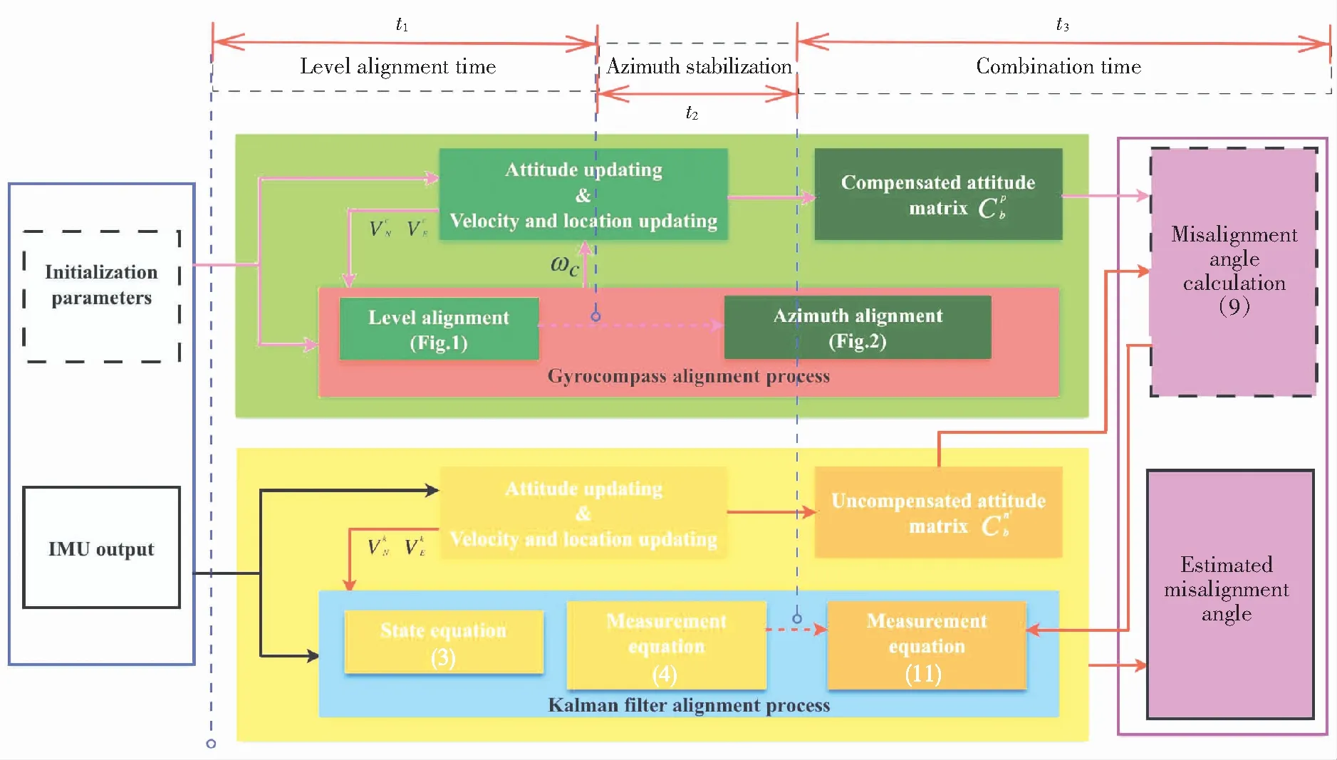
Fig.3 Structure diagram of the combined alignment mechanism

3.2 Analysis of the Combined Alignment Method

Because the rank of the system model represents the number of the observable state which can be estimated, it can qualitatively reflect the observability of the system. Since the observability of the system determines the convergence of the system state, the observability of the system model and the observable degree of the system state can be used to analyze the performance of the combined alignment method.

According to the discretization of the state space model for continuous time system, the observability matrix of the system model can be expressed by system transition matrixFkand measurement transition matrixHkas

(12)

wherenis the order of the system.

Based on the parameters setting in Section 4, the observability of the system model can be simply calculated through the rank of Eq.(12). Apparently, the ranks of the conventional KF alignment model, the ROKF alignment model, and the combined alignment model are 7, 5, and 5, respectively. Among them, only the rank of the conventional KF alignment model was less than the system dimension. To compare and analyze the observable degree of the system state variables, the eigenvalues and eigenvectors based on the system test matrix are introduced in this paper.

By the definition, the observable degree of the system model can be easily obtained. All the negative eigenvectors have been transformed to a positive plane for a clearer comparison. The eigenvalues and eigenvectors of the system models for the above three methods are shown in Figs.4-6.

The eigenvalue represents the observability of the state variable, and the observability determines the ability of the states to be estimated. As shown in Figs.4-5, only four state variables can be called “strong observable” and others are “weak observable” or unobservable. Thus, the horizontal velocity errors and the attitude misalignment angles can be easily estimated, whereas the azimuth misalignment angle is difficult to be estimated. It is quite obvious that the combined alignment model is fully observable, and all the observable degree is one for the state variables in Fig.6. The system model is fully controllable and observable, so the azimuth misalignment angle can be estimated.

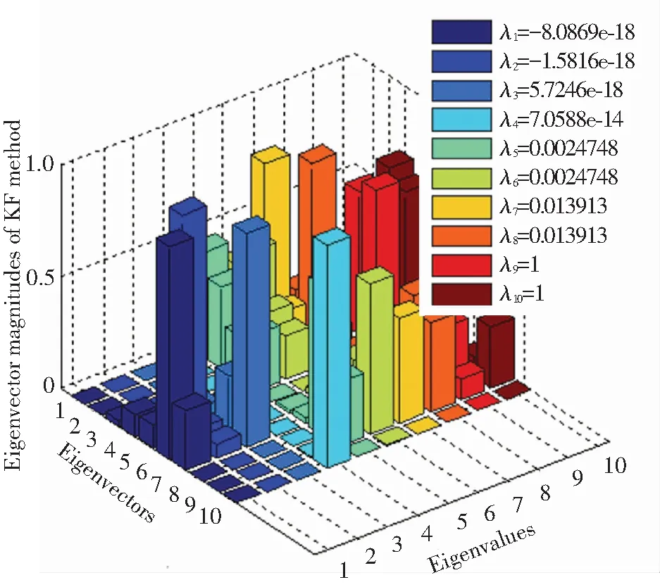
Fig.4 Eigenvalues and eigenvectors for conventional KF alignment model

Fig.5 Eigenvalues and eigenvectors for ROKF alignment model

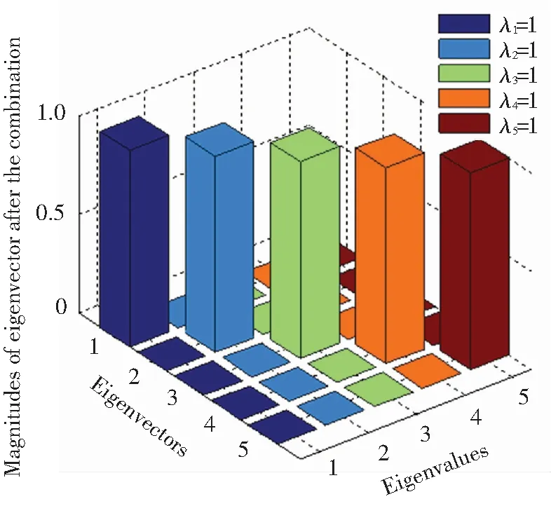
Fig.6 Eigenvalues and eigenvectors for the combined alignment model

In order to investigate the quantitative relationship between the KF alignment method and the gyrocompass alignment method, a brief angle relationship between the coordinate systems is shown in Fig.7.

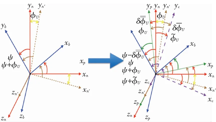
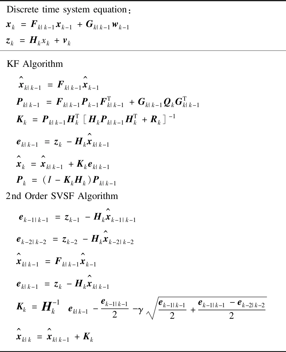
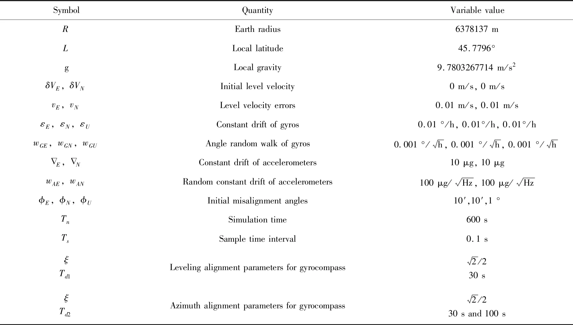
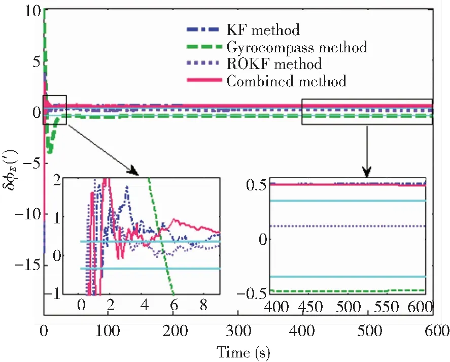
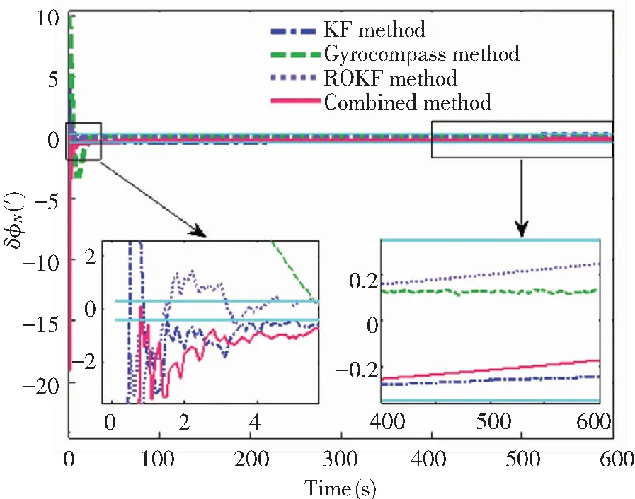
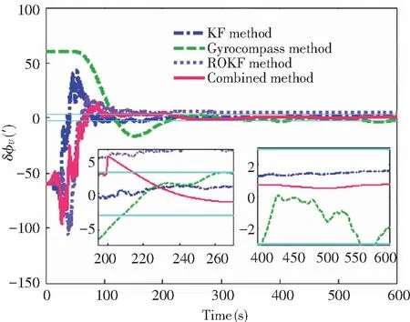
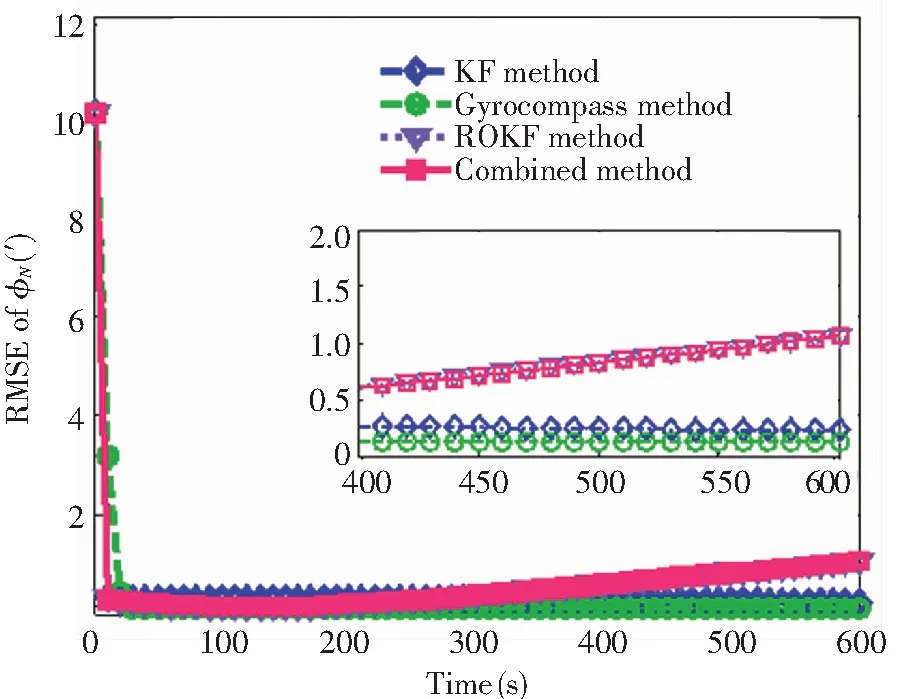
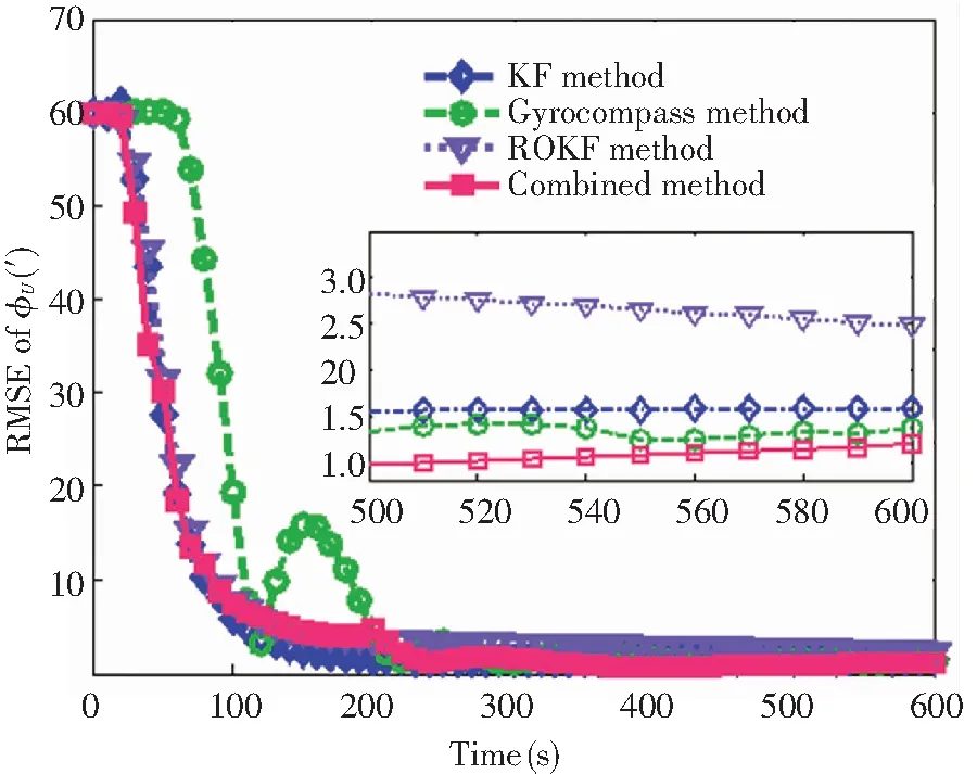
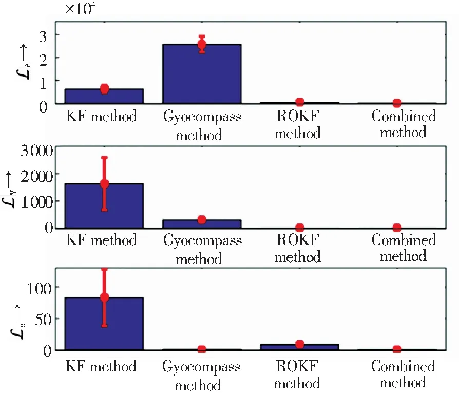
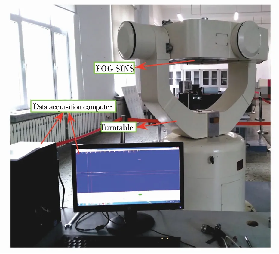
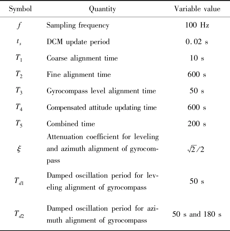
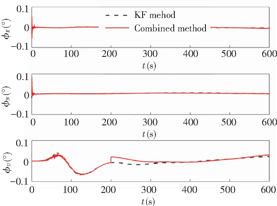
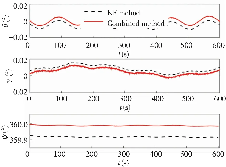
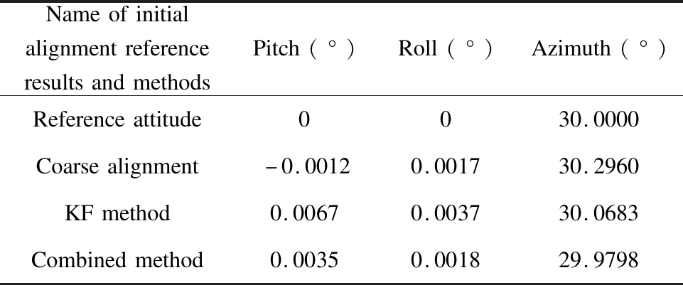
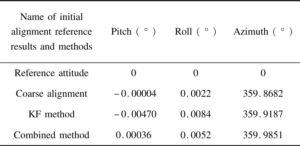
(a)t

According to Eqs.(7)-(8), the difference between the two types of alignment results is as follows:

(13)

Despite the introduction of the calculated misalignment angle, KF is not completely tracking the measurement state. The alignment result in the proposed method was similar to the mean of the estimation error from the KF alignment method and the gyrocompass alignment method. To illustrate the effectiveness of the combined alignment method, two filter algorithms, the KF method and the Second Order Smooth Variable Structure Filter (2nd SVSF) method, were used for discrete time system as shown in Table 1, which proved that the combined alignment method based on the KF algorithm was not just tracking. Here the combined alignment method is implemented by the two filtering algorithms in Table 1.

Table 1 KF and the 2nd SVSF algorithms

Since the results of the horizontal alignment are too small to easily conduct observation (Fig.8), the error result of the azimuth misalignment angle is only simulated and presented based on the simulation parameter in Section 4.

The 2nd SVSF is a model-based state estimation method and benefits from the robustness and chattering suppression characteristics of the second order sliding mode system[27], so the estimation error of the azimuth misalignment angle (solid line) is the same as the result of the gyrocompass alignment method (dashed) in Fig.8. Obviously, the combined alignment method based on the KF algorithm (dotted line) is not only tracking the measurement state, but makes the estimated error smaller and more stable. Compared with the combined alignment method based on the 2nd SVSF, the combined alignment method based on the KF algorithm was more accurate.

Fig.8 Comparison of two filtering methods for azimuth misalignment angle error

4 Simulation Results and Discussions

In this work, the numerical simulation of the combined alignment method was conducted based on the abovementioned combined alignment mechanism, and the simulation results were compared with the general alignment methods, including the conventional KF alignment method, the gyrocompass alignment method, and the ROKF alignment method. The statistical results and the negative log-likelihood analysis are used to evaluate the accuracy and consistency of the combined alignment method in this section. Similarly, the experimental test is implemented and the results are discussed.

4.1 Simulation Parameters Setting

The simulation parameters are listed in Table 2.

Table 2 Simulation parameters of initial alignment process

The initial parameters for the KF alignment method are expressed as follows:

State initial values:

X(0)=010×1

Error covariance matrix:

P(0)=diag([(0.1 m/s)2, (0.1 m/s)2, (10′)2, (10′)2, (1°)2, (10 μg)2,(10 μg)2, (0.01 °/h)2, (0.01 °/h)2, (0.01 °/h)2])

Process noise covariance matrix:

Measurement noise covariance matrix:

R(0)=diag([(0.01 m/s)2, (0.01 m/s)2])

The initial alignment parameters for the ROKF alignment method and the SVSF method are represented as follows:

State initial values:

X(0)=05×1

Error covariance matrix:

P(0)=diag([(0.1 m/s)2,(0.1 m/s)2,

(10′)2, (10′)2, (1 °)2])

Process noise covariance matrix:

Measurement noise covariance matrix:

R(0)=diag([(0.01 m/s)2,(0.01 m/s)2, 0, 0, 0])

4.2 Simulation Results and Discussions

The simulation process lasts for 600 s, and the combined alignment method can be operated according to Fig.3. To reveal the performance of the combined alignment method, several typical alignment methods are used to compare with the results, and the misalignment angle error curves are shown in Figs.9-11. The dash-dot line denotes the KF alignment method, dashed line denotes the gyrocompass alignment method, dotted line denotes the ROKF alignment method, and solid line denotes the combined alignment method. The parallel solid lines in zoom graphs represent the theoretical errors of the misalignment angle, which can be calculated by Eq.(7).

As shown in Figs.9-10, the ROKF alignment method had better pitch alignment accuracy than the other methods, and the gyrocompass alignment method had better roll alignment accuracy than other methods. However, the convergence speed of the gyrocompass alignment method was slower than those of other methods. The combined alignment method had the same convergence speed as the other methods including the gyrocompass alignment method. Although the combined alignment method did not achieve the best estimation accuracy in terms of horizontal misalignment angles, the estimation results were still better than those of the conventional KF method. Due to the azimuth stabilization process, the combined alignment method had a switching process which occurred at the moment of 200 s in Fig.11. It is obvious that the combined alignment method had a better estimation accuracy and stability. The azimuth misalignment angle error of the gyrocompass alignment method still occurred in the oscillation process, and the azimuth misalignment angle error of the ROKF alignment method exceeded the range of steady misalignment angle error.

Fig.9 Pitch misalignment angle error

Fig.10 Roll misalignment angle error

Fig.11 Yaw misalignment angle error

Because the state estimation process suffers from the uncertain influence of random noise existing in the system model, it lacks of comparability among the estimation methods using different noise. For the reason that 100 Monte Carlo runs have been performed to analyze the alignment results, the Monte Carlo averaging Root Mean Square Error (RMSE) of the estimation error for misalignment angles was analyzed (Figs.12-14).

The diamond represents the KF method, circle represents the gyrocompass method, downward-pointing square represents the ROKF method, and square represents the combined method. According to Figs.12-14, due to the role of the mean, the RMSE curves became smooth. From the result of alignment, the combined alignment method was not optimal (Figs.12-13), which was affected by the opposite of the steady state between Eqs.(7)-(8). In fact, only a number of times on average would have such a bad result, while those of others were not the worst. Since the combined method contains the gyrocompass method, the combined alignment method can obtain the horizontal alignment results from the gyrocompass alignment method which had the lowest RMSE (Figs.12-13). According to the analysis in Section 3.2, the estimation accuracy of the azimuth misalignment angle has been upgraded, thus resulting in a minimum RMSE (Fig.14).

Fig.12 RMSE of the pitch misalignment angle error

Fig.13 RMSE of the roll misalignment angle error

Fig.14 RMSE of the yaw misalignment angle error

For a clear contrast of the four methods, Fig.15 shows the Monte Carlo averaging of RMSE for the misalignment angle error between 400 s and 600 s. The RMSE of the pitch misalignment angle error for the four methods mainly settled on the neighborhood of 0.5′, the RMSEs of the roll misalignment angle error were different, and one of the best result occurred in the gyrocompass method. The combined method had the lowest RMSE of the yaw misalignment angle error, which was just two-thirds of the result of the KF method. Thus the combined alignment method could obtain the optimal alignment results, consisting of the horizontal alignment results from the gyrocompass method and the azimuth alignment results obtained by the combined estimation process.

Fig.15 Monte Carlo averaging of RMSE for the misalignment angle error (400 s-600 s)

In addition, the negative log-likelihood of the state estimation was introduced to penalize both inconsistency and uncertainty, which was the same as the RMSE that lower value indicates a better performance[28].

The comparative negative log-likelihood is shown in Fig.16, in which the subscript E, N, and U denote the pitch, roll, and yaw misalignment angle errors, respectively, and the histogram and error bar indicate the mean value and standard deviation of the negative log-likelihood, respectively. Although the combined alignment method did not obtain the best horizontal alignment result, it was the most consistent and had no uncertainty in the 100 Monte Carlo simulations. Thus, the combined alignment method provides a novel estimation form, and receives better estimation result of the azimuth misalignment angle in the case that there is no loss of horizontal alignment accuracy because of the usage of the gyrocompass horizontal alignment result.

Fig.16 Negative log-likelihood of four methods

5 Experimental Test Results and Discussions

The merits of the combined alignment method have been analyzed by numerical simulation test in Section 4. The data acquisition experiment using turntable is conducted in this section, so that the applicability and estimation accuracy of the combined alignment method can be confirmed by the alignment result of the actual inertial sensor data. In the data acquisition experiment, the FOG SINS, data acquisition computer, and turntable were used (Fig.17).

Fig.17 Data acquisition devices

The FOG SINS was fixed on the turntable, and the attitude reference was given by the high-precision turntable with thermostatic box that the wobble error was less than 2″, the position error was less than 3″, and the rate resolution was 0.000 1 °/s.

In the data acquisition experiment, a total of two sets of data were collected. In order to maintain the consistency with the simulation process, the first set of data was collected based on 30 ° azimuth angle and 0 ° horizontal attitude angle. The second set of data was used to verify the north finding capacity of SINS, so that the horizontal attitude angle and the azimuth angle were both zero. Two sets of data were collected for half an hour and the sampling frequency was 100 Hz. The FOG SINS used the KF method as the alignment method of the SINS, and the optimal alignment accuracy was 0.06 °. Some system parameters of the initial alignment process should be changed to apply to the self-made SINS. The other system parameters were the same as those in Table 2. Table 3 shows the parameters that need to be changed.

Table 3 Changed parameters of the system

The initial error covariance matrix for the KF alignment method is represented as follows:

P(0)=diag([(0.2 m/s)2,(0.2 m/s)2, (1 °)2,

(1°)2, (1 °)2, (10 μg)2,(10 μg)2,

(0.01 ° /h)2, (0.01 °/h)2,

(0.01 °/h)2])

The initial error covariance matrix for the ROKF alignment method and the combined alignment method are represented as follows:

P(0)=diag([(0.2 m/s)2, (0.2 m/s)2,

(1 °)2, (1 °)2, (1 °)2])

The other filter parameters are the same as those in Section 4.

To illustrate that the combined alignment method can refine alignment accuracy,it was compared with the KF alignment method of self-made SINS. First of all, the same analytic coarse alignment of timeT1was carried out. Then the fine alignment of timeT2was conducted based on the above results, and the combined alignment process was still experimented after timeT5. In the end, DCM was corrected after the fine alignment process, and the compensated attitude angle and the azimuth angle of timeT4were recorded to evaluate the estimation performance of two fine alignment methods. The initial alignment process and the compensated results, in the case of azimuth angle of 30 ° and azimuth angle of 0 °, are shown in Figs.18-21.

Fig.18 Fine alignment process results (azimuth angle of 30°)

Fig.19 Attitude compensated results (azimuth angle of 30°)

Fig.20 Fine alignment process results (azimuth angle 0°)

Fig.21 Attitude compensated results (azimuth angle 0°)

The ordinate variablesφE,φN,φU,θ,γ, andψin the figures represent the pitch misalignment angle, roll misalignment angle, azimuth misalignment angle, compensated pitch angle, compensated roll angle, and compensated azimuth angle, respectively. The unit of ordinate angle is degree, and the abscissa is the timetin seconds.

In Figs.18-21, the KF alignment method and the combined alignment method had the same estimation trajectory before timeT5, and after that there was an obvious switching process in the combined alignment method. Actually, the more obvious the switching process is, the bigger the error between the gyrocompass alignment method and the ROKF alignment method is. Apparently, the azimuth angle convergence rates in Figs.18-21 were much slower than those in Figs.9-11, whose sampling time was only 0.1 s. Apart from the simulated Inertial Measurement Unit (IMU) data, the performance of the fiber gyroscope or the actual IMU data which was mixed with various inside interference made the alignment results worse. Thus, the result of the initial alignment process is hard to obtain, which was perfectly consistent with the numerical simulation. Due to the impact of gyroscope performance, a slight oscillation occurred after the switching process (Fig.18), because the convergence rate of the gyrocompass alignment method became slow. The estimation curve is relatively stable in Fig.20, so the alignment results of the combined alignment method would be closer to the simulation results in Figs.9-11. The numerical results for the initial alignment process are shown in Tables 4-5.

Table 4 Numerical results for the initial alignment process(azimuth angle 30°)

Table 5 Numerical results for the initial alignment process(azimuth angle 0°)

In Tables 4-5, the results of the fine alignment process are the average values of the compensated horizontal attitude angle and the azimuth angle, respectively. Compared with the reference value, the azimuth alignment accuracy of the combined alignment method was 1.212′ and 0.894′, which were higher than 4.098′ and 4.878′ in the KF alignment method, and was the same for the horizontal attitude angles. Through the comparison of the same set of data, the combined alignment method had more obvious advantages than the KF alignment method, and the alignment process and the results were all close to the results of the numerical simulation. Thus the combined alignment method is feasible and practical, and it has good consistency with the numerical simulation process.

6 Conclusions

A combined alignment mechanism is proposed in this paper to refine the estimation accuracy of the azimuth misalignment angle. The combined alignment model was formulated, and the combined alignment strategy was analyzed based on the observability analysis and the mathematical deduction. In order to confirm the correctness and practicability of the theoretical analysis, 100 Monte Carlo simulation runs were carried out, and RMSE and negative log-likelihood calculation were used to evaluate the performance in terms of accuracy and consistency of the estimation results. The simulation results showed that the combined alignment method could effectively enhance the estimation accuracy of the azimuth misalignment angle. Although the horizontal alignment result was not better than those of other comparative methods, the horizontal alignment accuracy would not become worse due to the use of horizontal alignment result from the gyrocompass alignment method. Additionally, the data acquisition and the initial alignment experiment were conducted to confirm the practicability and consistency of the combined alignment method. The convergence speed is not further considered for improvement in this paper, because an alignment method based on the storage of IMU data can effectively reduce the alignment time which has been used in the KF alignment method and the gyrocompass alignment method. Since the combined alignment method is based on the ROKF alignment model and the strapdown gyrocompass alignment model, the improvement of the alignment time for the combined alignment method can be easily accomplished through the data storage method.