ITˆO DIFFERENTIAL REPRESENTATION OF SINGULAR STOCHASTIC VOLTERRA INTEGRAL EQUATIONS∗

Nguyen Tien DUNG

Division of Computational Mathematics and Engineering,Institute for Computational Science,Ton

Duc Thang University,Ho Chi Minh City,Vietnam

Faculty of Mathematics and Statistics,Ton Duc Thang University,Ho Chi Minh City,Vietnam

E-mail:nguyentiendung@tdtu.edu.vn

Abstract In this paper we obtain an Itˆo differential representation for a class of singular stochastic Volterra integral equations.As an application,we investigate the rate of convergence in the small time central limit theorem for the solution.

Key words stochastic integral equation;Itˆo formula;central limit theorem

1 Introduction

Let(Bt)t∈[0,T]be a standard Brownian motion defined on a complete probability space(Ω,F,F,P),where F=(Ft)t∈[0,T]is a natural filtration generated byB.It is known that stochastic Volterra integral equations of the form

play an important role in various fields such as mathematical finance,physics,biology,etc.Because of its applications,the class of stochastic Volterra integral equations has been investigated in several works.Among others,we mention[2,11]and references therein for the existence and uniqueness of solutions,[4]for comparison theorems,[8,10]for stability results,[6]for perturbed equations,[7]for numerical solutions.

One of main difficulties when studying the properties of(1.1)and related problems is that we can not directly apply Itˆo differential formula to(1.1).In the case of the equations with regular kernels,we can avoid this difficult by rewriting(1.1)in its Itˆo differential form.In fact,we have

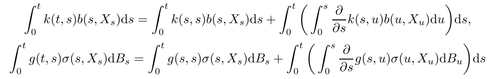
and we obtain the following Itˆo differential representation

whereX

Generally,this nice representation does not hold anymore if the kernels are singular,except we imposed additional conditions.The case,where the kernelg(t,s)is singular,has been discussed in our recent work[3].We have to use the techniques of Malliavin calculus to obtain an Itˆo-type differential transformation involving Malliavin derivatives and Skorokhod integrals,it is open to obtain an Itˆo differential representation for the solution in this case.The aim of the present paper is to study the case,where the kernelk(t,s)is singular.

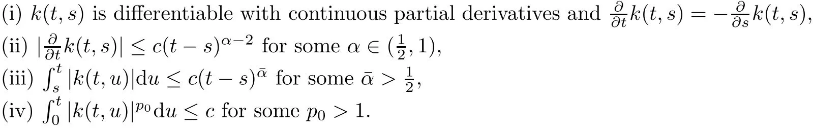
In the whole paper,we require the assumption:

(A1)The kernelk(t,s)is defined on{0≤s0,

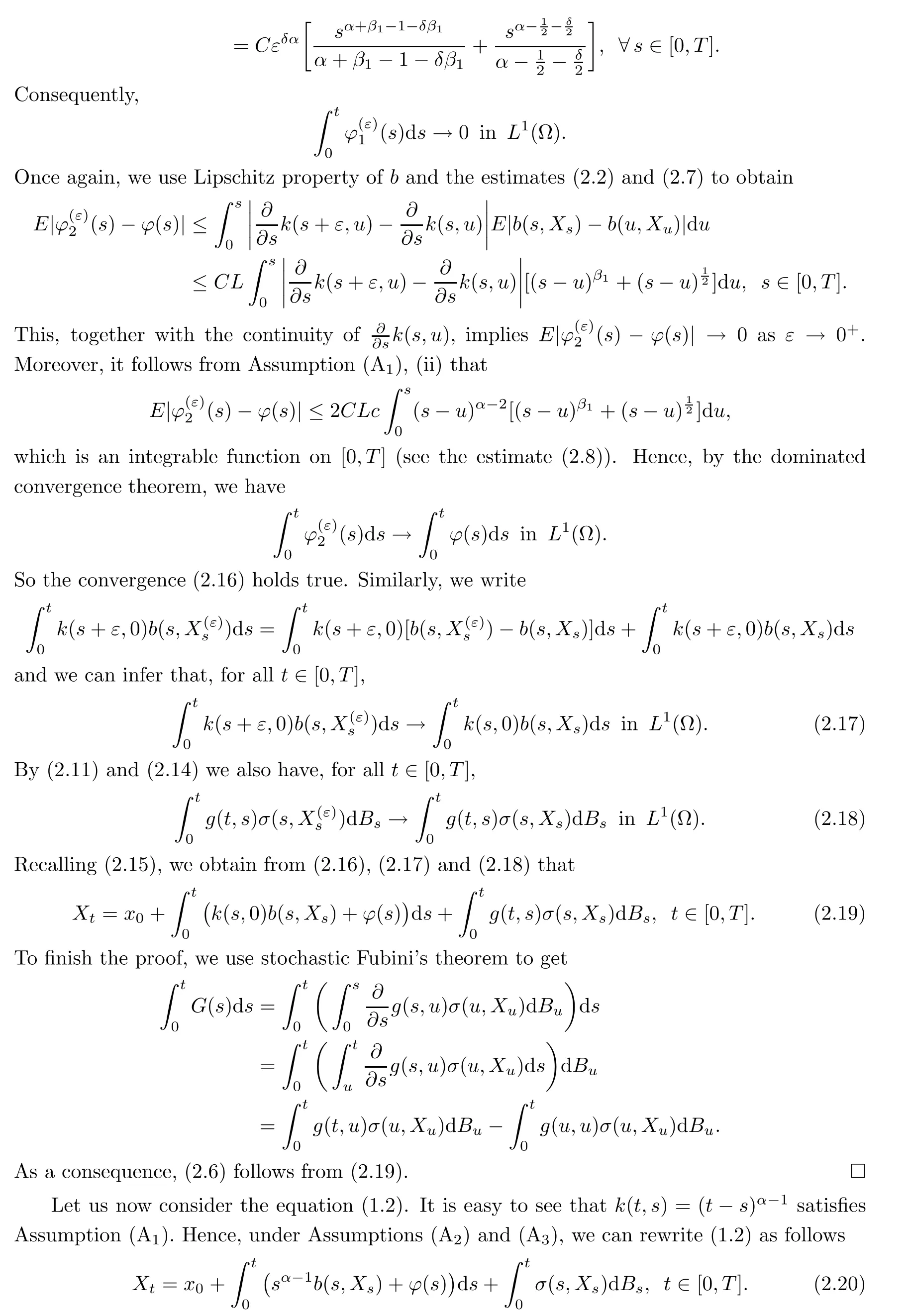
Under(A1)and regular conditions onb,σandg,we are able to obtain a nice Itˆo differential representation for the solution in Theorem 2.2.This representation allows us to use Itˆo differential formula for studying deeper properties of the solution.As a non-trivial application,our Theorem 2.3 provides an explicit bound on Wasserstein distance in the small time central limit theorem for singular stochastic Volterra integral equations of the form

wherex0∈R andα∈(12,1).Here we setk(t,s)=(t−s)α−1to illustrate the singularity ofk(t,s)andg(t,s)=1 for the simplicity.We also note that the small time central limit theorem is useful particularly for studying the digital options in finance,see e.g.[5].

2 The Main Results

In the whole paper,we denote byCa generic constant,whose value may change from one line to another.Since our investigation focuses on the singularity ofk(t,s),we are going to impose the following fundamental conditions onb,σandg.

(A2)The coefficientsb,σ:[0,T]×R→R are Lipschitz and have linear growth,i.e.,there existsL>0 such that:

and

The kernelg:[0,T]2→R is differentiable in the variablet,and bothg(t,s)andare continuous.

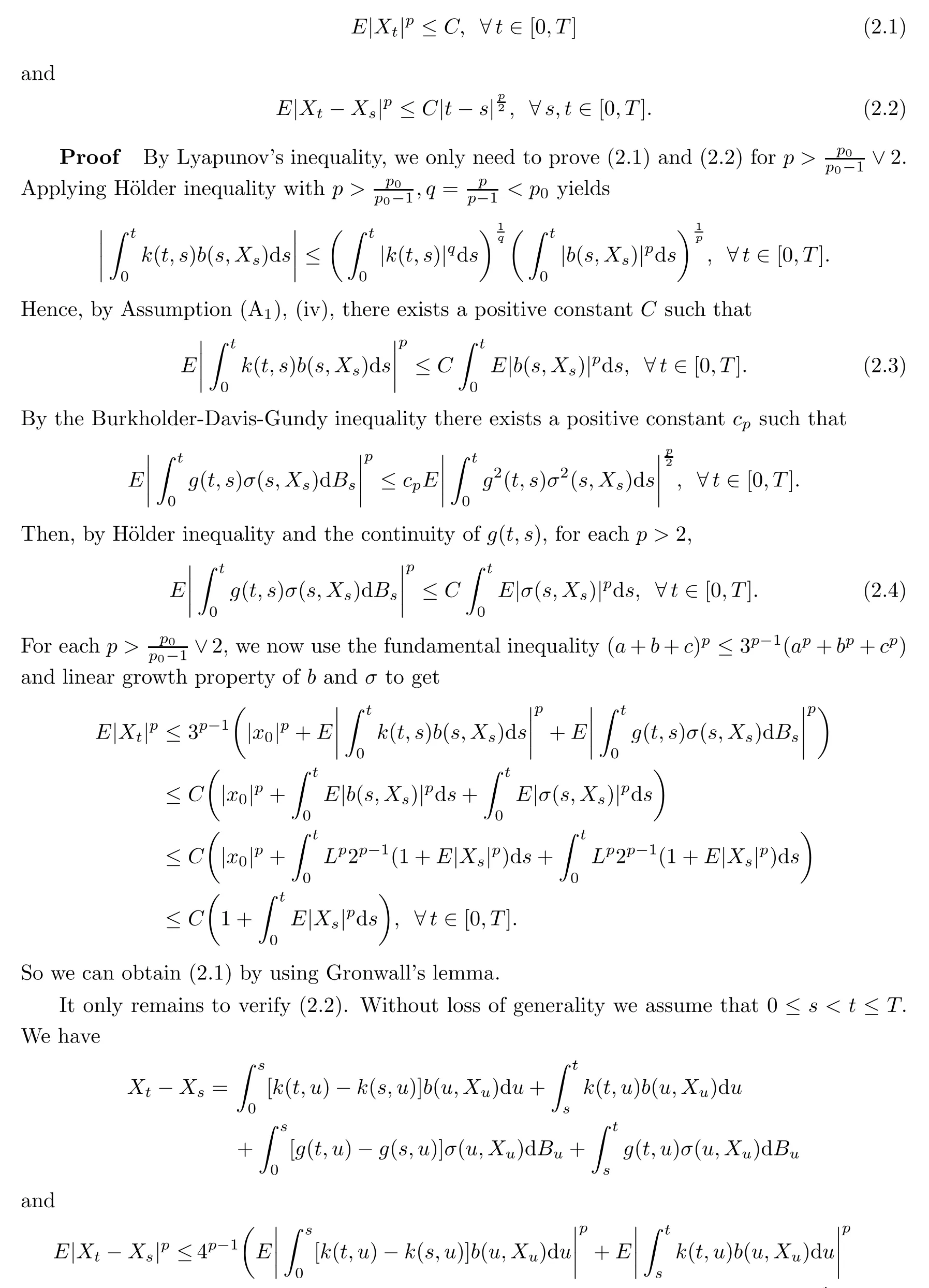
Proposition 2.1Let(Xt)t∈[0,T]be the solution of the equation(1.1).Suppose Assumptions(A1)and(A2).Then,for anyp≥1,there exists a positive constantCsuch that

which leads us to(2.2)becauseα,¯α>.This completes the proof.

We now are in a position to state and prove the first main result of the paper.To handle the singularity ofk(t,s),we need to additionally impose the following condition.

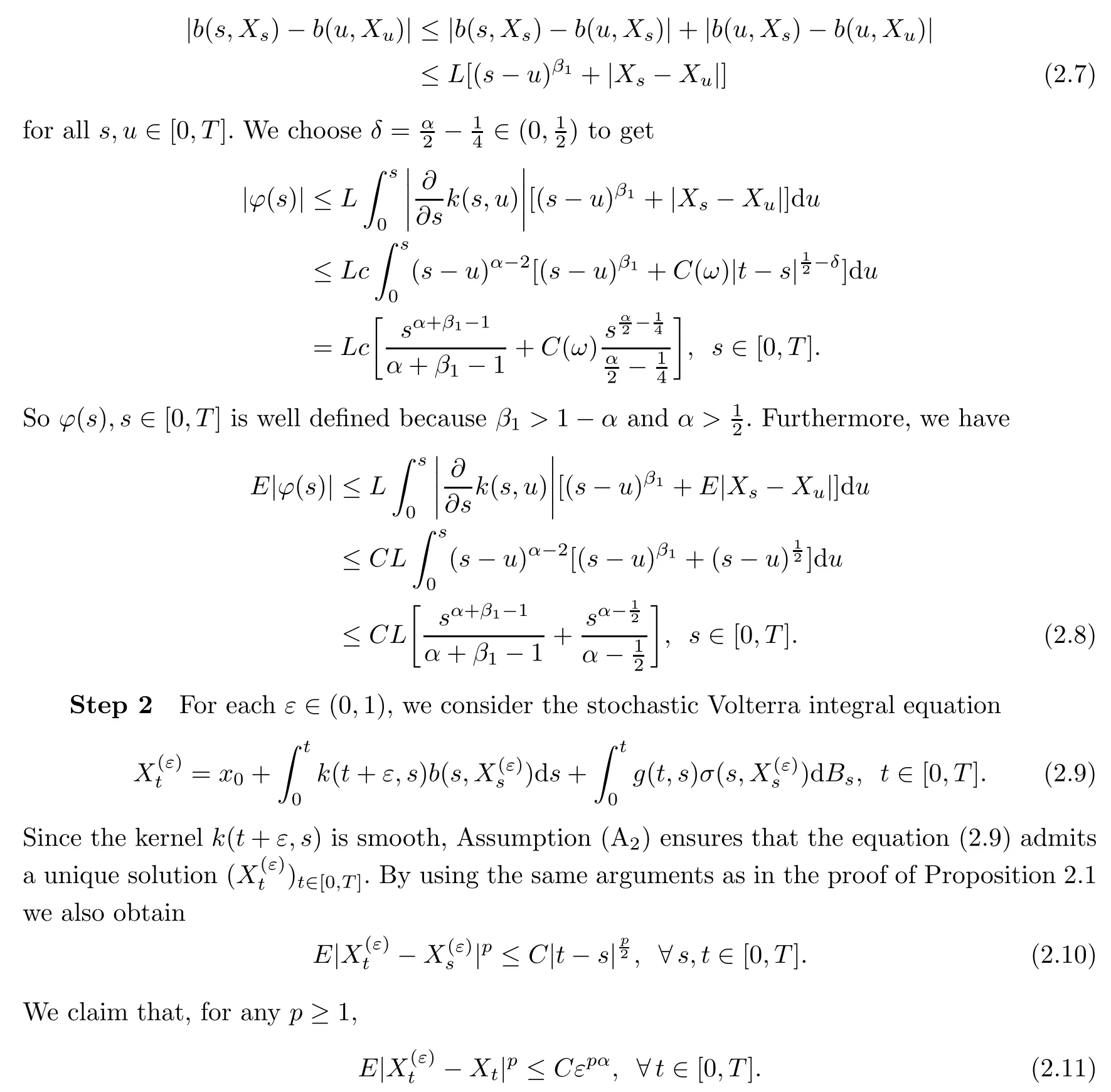
(A3)Givenαas in Assumption(A1),(ii).There existsβ1>1−αsuch that

Theorem 2.2Suppose Assumptions(A1),(A2)and(A3).The solution(Xt)t∈[0,T]of the equation(1.1)admits the following Itˆo differential representation

ProofWe separate the proof into four steps.

Step 1We first verify thatϕ(s),s∈[0,T]is well defined.By Kolmogorov continuity theorem,it follows from(2.2)that for anythere exists a finite random variableC(ω)such that

By Lipschitz property ofband Assumption(A3)we deduce

Here we emphasize that the constantsCin(2.10)and(2.11)do not depend onε∈(0,1).We have

We use H¨older inequality to get,for anyp>1,

By using the same arguments as in the proof(2.3)we obtain,for anyp>

By using the same arguments as in the proof(2.4)we obtain,for anyp>2,

or equivalently

Inserting this relation into(2.9)gives us

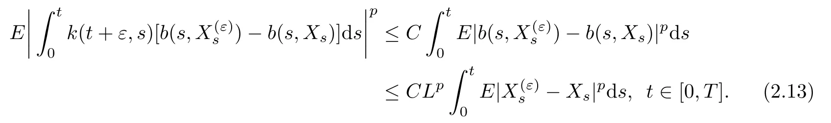
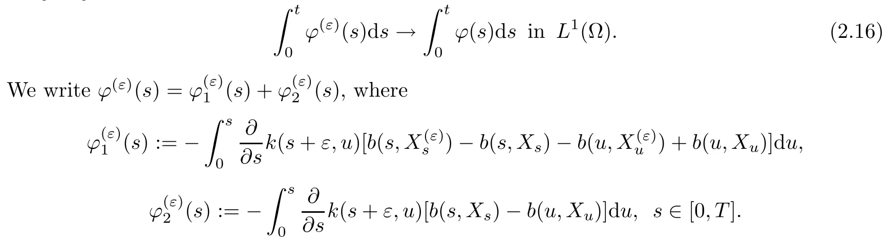
Step 4This step concludes the proof by lettingε→0+.We first show that,for allt∈[0,T],

By Lipschitz property ofband the claim(2.11)we deduce

On the other hand,we deduce from the estimates(2.2),(2.7)and(2.10)that

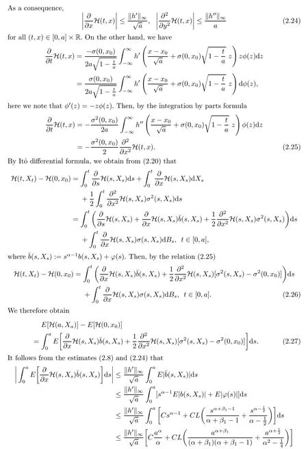
Minimizing inu,the right hand side of(2.30)attains its minimum value atu0:Whena→0+,we haveu0∈(0,).So the conclusion follows substitutingu0in(2.30)and then taking the supremum over allh∈C1with∞≤1.

The proof of Theorem is complete.