Effect of background fluctuation on velocity diagnostics by Mach probe
2020-12-02YunxiaoWEI魏云逍andZheGAO高喆
Yunxiao WEI (魏云逍) and Zhe GAO (高喆)
Department of Engineering Physics, Tsinghua University, Beijing 100084, People’s Republic of China
Abstract
Keywords: velocity diagnostics, Mach probe, electrostatic fluctuation
1.Introduction
Since the 1990s, effects of plasma toroidal rotation on the behavior of plasma were found on multiple tokamak devices.It was shown that moderate plasma rotation could stabilize plasma [1, 2] and thus could help to achieve higher parameters; afterwards, the discovery of intrinsic rotation further stimulated research interests [3].It is believed that plasma rotation will play a key role in next-generation magnetic confined fusion reactors [4].Concerning the physics of plasma rotation, there have been theories from different aspects, i.e.momentum [5], angular momentum [6] and velocity [7], etc.On the other hand, to experimentally investigate the plasma rotation,it is mandatory to measure the plasma velocity.Various velocity diagnostic approaches have been developed, such as Mach probe [8], Doppler effect of CXRS (Charge-eXchange Recombination Spectroscopy) [9]and velocimetry based on TDE(Time Delay Estimation)[10],etc.
In principle,to verify these theories of plasma rotation by experiments, it is necessary first to specify the physical essence of the quantity determined from the diagnostics.Usually, the models of velocity diagnostics are based on the hypothesis of uniform density background,where the velocity and momentum are equivalent.However, when density fluctuation exists in turbulent plasma, a deviation could emerge.If we split the physical quantities into average part and fluctuation part, i.e.n=n+n, then, for example, the effective velocity deduced from mean momentum flux is

which deviates from the true mean velocityby a coupling vale of density fluctuation and velocity fluctuationWhen dealing with a highly turbulent process,like radio frequency waves current driving [11], such coupling value is non-negligible.Despite progress made in theoretical and experimental researches on plasma rotation separately,the distinction between different‘speed’quantities has been ambiguous,and diagnostics cannot distinguish them.Such ambiguity can cause confusion.Taking Doppler effect as an example, it is well known that the wavelength shift is proportional to particle velocity:one may suppose Doppler effect can be employed to measure the mean velocity directly, but it turns out that it actually gives the mean flux, as shown in the appendix.Therefore, it is meaningful to discuss how velocity diagnostics would be affected in the case of non-uniform background.
In the present work we studied the case of Mach probe(MP),a classical and widely-used Langmuir probe diagnostic,in the kinetic one-dimensional electrostatics regime following Chung[12].In section 2 the basic configuration and physical model of MP is introduced, a model of background electrostatic wave is constructed and discussed in section 3, the effect of such fluctuation on MP is calculated in section 4,and finally section 5 gives a summary.
2.Kinetic model of MP measurement
A typical MP is composed of two directional electric probes located at opposite sides of a common insulator between them,and both probes collect the ions in the parallel direction with respect to the plasma flow or the magnetic field directions; the probes are negatively biased enough to collect the ion saturation current [8].In typical tokamak plasma, it was found that the flow Mach number was related to upstream and downstream collected current’s ratio by a simple exponential relation

Several theoretical models of such magnetized MP have been proposed since the 1980s, such as fluid models by Stangeby [13] and Hutchison [14], and the kinetic model by Chung and Hutchinson[12,15].The center of the debate was on how to consider the cross-field transportation, especially the viscosity-to-diffusivity ratioIt was found thatα~ 1 is in better accordance with LIF experiment [16],corresponding to exponential relation anduc~0.6(inTi=Tecondition).From then on this value has been widely used in MP experiments in various devices such as tokamak [17],spherical tokamak [18] and stellarator [19].Notice that in some works the Mach number is calculated viainstead ofVs.
The typical kinetic model of MP considers ions’ movement along the presheath as primary, while it takes into account the cross-field transport by introducing a source term related to‘exchange rate’W into the ion Boltzmann equation.The electrons are assumed to be isothermal and described by the Boltzmann relation.In a one-dimensional and electrostatic system, the normalized model equations for ion distribution function and potential profile in the presheath can be described as
where we normalize velocity by ion sound speedlength by presheath characteristic lengthdensity by mean background densityand energy(potential as well)by electron temperatureis background plasma distribution function.When background plasma is uniform and Maxwellian,ucis only determined by background temperature,1, 0.2 yieldinguc=0.54, 0.61, 0.78.
3.Background electrostatic fluctuation wave
In order to investigate the effect of background fluctuation on MP, we introduce electrostatic fluctuation into the kinetic model of MP, equations (3)-(5).When fluctuation exists, the backgroundf∞(x,u)is no more uniform in x nor Maxwellian in v.By substitutingf=f∞,equation(3)reduces to a Vlasov equation, thus equations (3)-(5) constitute a Vlasov-Poisson problem, which is intrinsically nonlinear and is a basic but important question for plasma dynamics.Solving the problem, we can obtain the distribution functionf∞(x,u) and potential profileφ∞(x) of background plasma.
A solution to this problem(BGK mode)is constructed by Bernstein et al[20].The basic idea is to divide the particles of different species into free partsfif,fefand trapped partsfit,fet,then prescribe the functions except one in accordance with the Vlasov equation, and finally calculate the remaining one by the Poisson equation;thus both equations are satisfied.There are two methods: one is to prescribeφ(x),fi,fefand calculatefet,with which the Poisson equation is an integral equation and could be solved by deconvolution method [21];the other is to prescribefi,feand calculateφ(x) ,with which the Poisson equation is a differential equation and could be solved by pseudopotential method [22].
Our goal is to evaluate the response of MP under background plasma with various flow speed and fluctuation wave amplitude, so it is required that amplitude and speed can be prescribed independently.Then, in order to stay consistent with the MP model, it is necessary that electrons satisfy the Boltzmann relation,the ion flux is constant and the fluctuation is periodical.In such a case, the second method is more favorable.Finally,in the limit of zero fluctuation,the solution should go back to being uniform and Maxwellian.Therefore,we prescribe the normalized ion distribution function as

where quantities are normalized as the previous section,except that density is normalized to electron density atφ=ψ,yielding normalization constant A; the value range ofφisφ∈ [0,ψ],ψis peak-peak value of potential wave;u0is macro speed parameter;θ=Te/Tiis temparature ratio,is the boundary of free and trapped ions,αis trapped ion negative temparature parameter;κ=φ′′∣φ=ψmust be nonzero to make fluctuation periodical and is taken as− 10−3in the present paper.Normalized electron density isne(φ)=exp(φ−ψ).
The zeroth moment of equations (6) and (7) yields normalized ion density:

where I denotes the free symmetrical part, K denotes the free non-symmetrical part related tou0and Q denotes the trapped part related toα, defined as [21, 22]

The first moment of equations (6) and (7) yields normalized ion flux:

which is proportional tou0and is constant as required.
The pseudopotential method is to define pseudopotentialand finally yields the inverse function of potential profileφ(x):

This yields a monotone half of the wave.Assuming it starts at(x0,φ0) =(0, 0) and ends in(xm,ψ) ,the periodical condition requires thatφ′(x0)=φ′(xm)=0,i.e.V(0)=V(ψ)=0.V(0)=0is evident, whileV(ψ)=0gives the‘dispersion relation’ between the parametersθ,ψ,u0,α,if we prescribeθ,ψ,u0,thenαis determined, and thus the potential profile and ion distribution function can be determined.In this paperθis taken asθ= 5, results with otherθare similar.
However, it turns out that(ψ,u0) cannot be prescribed arbitrarily.In the present modelV(φ)<0 forφ∈(0,ψ)turns out to be a pretty strong requirement, limiting the parameters to an ‘allowed zone’, as shown in figure 1.When fluctuation amplitudeψ→0 there is little restriction onu0;but in the case of finite fluctuation amplitude the parameters are restricted to a circle-like zone with a radius of roughly 0.8.Such restriction is related to the assumed simple model of trapped distribution functionfit.Noticing thatfitdoes not provide macro flux and vanishes in the limit of zero fluctuation, so in principle we can manipulatefitfreely, maybe some model offitcould avoid such a limited allowed zone;or maybe it is indeed a physical limitation.

Figure 1.‘Allowed zone’ of parameters(ψ, u0) forθ = 5, given by the requirement V(φ)<0 for φ∈(0, ψ).
In the allowed zone we can calculateφ(x) ,fi(x,u) ,ni(x)profile.The fluctuation wave has the property that the wavelength is at the magnitude of 101λD,the waves of potential and density share the similar normalized amplitude(~ψ/ 2),and are in-phase,which means that there are always fewer ions inside the potential well where the energy is negative compared to free ones, which is whyαis called the negative temparature parameter.From equation(12)we know that the normalized flux increases withψ.
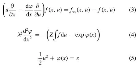
Now we look into the difference betweenu1= 〈Γ〉 /〈n〉(effective velocity deduced from mean momentum flux with mean density) andu2= 〈Γ /n〉(real mean velocity),D=u2/u1−1with respect to(ψ,u0) is plotted in figure 2.D(ψ) shows a quadric tendency, as indicated in equation (1)that the difference is fundementally quadratic to fluctuation amplitude; due to the limited allowed zone, the calculation stops at finite amplitude, but we can expect the difference continues to grow;at high fluctuation it is expected to become considerable.On the other hand,D(u0) shows a mild but obvious decreasing tendency, indicating the influence on MP fitting parameteruc,asucis deduced from data at variousu0,despite the fact that the difference itself is rather small.
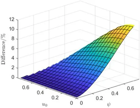
Figure 2.The relative difference between effective velocity deduced from mean momenteum flux with mean density u1= 〈Γ〉 /〈 n〉and real mean velocity u2= 〈Γ/n〉 ,i.e.D =u2/u1−1,in terms ofpercentage, vary with(ψ,u0).θ = 5.
4.Effect of the fluctuation on MP measurement
Now we apply the resultant electrostatic waves as background fluctuation to the MP model.Using the iteration method following Chung[12],the ion presheath distribution function profiles in the presence of electrostatics fluctuation waves are obtained numerically.
A sample off x u,()is shown in figure 3,where a unique phenomenon of discrete thin lines in phase space is illustrated(figure 3(b)) in contrast with the case without fluctuation(figure 3(a)).This is made possible by stair-like potential peaks near the adequately biased probe combined with the trapped ion negative temparature parameter: because of the‘negative temperature’ inside and the positive temperature outside, a density spike is formed on the brink energy of potential well (corresponding to±utin equation (6)), so the ions with brink energy overwhelmed others with nearby energy and outstood in the phase space, forming a discrete thin line on the phase space diagram when flowing into the probe; every line contains ions on the same energy orbit, so we may also call such lines ‘visualization of energy orbit’.That is to say, the collected flow is constituted of somehow discrete energies rather than a continuous spectrum as in the case without fluctuation.Such a phenomenon is affected by the shape of potential stair andu0as well,so an impact on the MP diagnostics could be expected.
Then the collected flowsΓw(absolute value)with respect to(ψ,u0) are calculated and plotted in figure 4.Besides the evident fact thatΓwdecreases withu0,the influence ofψis interesting:onu0=0.47theΓwis approximately independent ofψ,corresponding to the horizontal line(u0,Γw) =(0.47, 0.29),whereas the rest of the surface is subtly rotated alongψaround this line.The unparalleled lines ofΓw(u0) at variousψmake clear the fact thatucis dependent ofψ.

Figure 4.Plot of collected currentΓw( ψ,u0) in the allowed zone.θ = 5.
Now we defineu1,u2as previous sections, and calculate the fitting constant for eachuj:

the result underθ= 5 is shown in figure 5.As expected, at small fluctuation bothucjconverge to the reference valueuc0=0.536,while whenψ( peak-peak value of normalized fluctuation wave)rises,both of them increase to deviate fromuc0.That is to say, if we apply theuc0obtained in non-fluctuation condition when measuring the flow with fluctuation,the quantity we get will be less than the actual value, but is always closer torather than
Inside the allowed zone,we may obtain a fitting function for bothu cj(ψ) as

Figure 5.Diagram ofu cj (ψ),j=1, 2and their fitting curve and extrapolation outside the allowed zone; the reference value without fluctuation u c0=0.536is also shownθ = 5.
where(a1,b1) =(0.410, 2.88)and(a2,b2) =(0.614, 2.57).As we can see, the power parameterbjis rather big, noting a rapid nonlinear growth ofucjwhen generalized to high amplitude fluctuation cases,as is illustrated with dashed lines in figure 5.In typical tokamak plasma, especially in the edge region when MP is deployed, the density fluctuation can benr>50%[23], corresponding toψ≥1,.At this point the error betweenuc1anduc0(namely between actualv1and miscalculatedv0) can bee=uc1/uc0− 1 ≥40%,which is quite considerable even compared to the rough accuracy of MP diagnostics; thus a major correction is considered necessary.
However, because of the aforementioned ‘allowed zone’problem, the actual calculation stopped atψedge= 0.8,so such extrapolation becomes less convincing whenψis too far from theψedge:there may be other mechanism,say saturation,at high amplitude.
5.Summary
In summary, the effect of background fluctuation on velocity diagnostics, especially by Mach probe, is studied.The connection and distinction between different‘speed’quantities in theories and experiments are discussed,and then,the essence of velocity diagnostics is revisited, especially when the fluctuation exists.
In this paper,the impact of background fluctuation on ion presheath distribution function profile, collected flow, and,therefore, the MP fitting parameterucare calculated.It is found that, if we overlook the fluctuation and use theuc0obtained under uniform background hypothesis to derive the speed, the velocity will be underestimated, although it is always closer to(effective velocity deduced from mean flux)rather than(real mean velocity).=(0.410, 2.88) ,the deviation To measure, a fitting function foruc(ψ) is obtained:betweenucanduc0can hit 40% when density fluctuation is 50%,indicating the necessity of correction at high fluctuation level.
However, such a calculation is available only in an allowed zone discussed in section 3.This restriction is related to the model we use, we proposed to manipulate the form of trapped ions’distribution function to steer away from it,while it is also possible that it is actually a physical restriction.This problem remains open and to be further studied.On the other hand,there are many other types of fluctuation besides the 1D electrostatic wave model employed here, and so more complicated effects of fluctuation on the velocity diagnostics may be expected.
Acknowledgments
This work was supported by National Natural Science Foundation of China (Nos.11827810 and 11875177), International Atomic Energy Agency Research Contract No.22733 and the National Ten Thousand Talent Program.
Appendix.Doppler effect diagnostics under fluctuation
We assume a rough one-dimensional model to check the essence of Doppler effect.Assuming that the light intensity is proportional to ion amount in the detection regionwheref z v,()is measured ion distribution function andC0,C1are taken as constant,we can get the spectrum distribution

For conciseness, we take the velocity corresponding to spectrum peak as the measuredveff[24], namely

then assume ion is Maxwellianwhere temperature is taken as constant, equation (A.2) gives

It is shown that Doppler effect diagnostics gives mean momentum flux rather that mean velocity of particles, even though it reflects actual velocity of every single particle.In the presence of density fluctuation such two speed quantities are not equivalent, whereas experimentalists usually confuse them.
杂志排行

Plasma Science and Technology的其它文章
- The structure of an electronegative magnetized plasma sheath with non-extensive electron distribution
- The effect of forced oscillations on the kinetics of wave drift in an inhomogeneous plasma
- Numerical simulation of impact of supersonic molecular beam injection on edge localized modes
- Mitigation of blackout problem for reentry vehicle in traveling magnetic field with induced current
- New method for rekindling the explosive waves in Maxwellian space plasmas
- Molecular dynamics simulations of the interaction between OH radicals in plasma with poly-β-1-6-N-acetylglucosamine