Quantitative analysis modeling for the ChemCam spectral data based on laserinduced breakdown spectroscopy using convolutional neural network

Xueqiang CAO(曹学强),Li ZHANG(张立),Zhongchen WU(武中臣),Zongcheng LING(凌宗成),Jialun LI(李加伦) and Kaichen GUO(郭恺琛)

1 School of Mechanical,Electrical & Information Engineering,Shandong University,Weihai 264209,People’s Republic of China

2 Shandong Provincial Key Laboratory of Optical Astronomy and Solar-Terrestrial Environment,Institute of Space Sciences,Shandong University,Weihai 264209,People’s Republic of China

Abstract

Keywords:laser-induced breakdown spectroscopy,convolutional neural network,activation function,optimization method,quantitative analysis

1.Introduction

As a powerful and convenient technique,laser-induced breakdown spectroscopy(LIBS)has been utilized to analyze the spectrum with multivariate regression algorithms in order to obtain the relative content of each compound in samples.So far,LIBS has been widely applied to many geochemical fields with the advantages of convenient operation and high working efficiency[1].Due to the miniaturization,the handheld LIBS analyzer has also been adopted to analyze iron,rock and other materials[2,3].Furthermore,considering it can characterize target chemistry remotely and rapidly,LIBS has also been successfully used in situ quantitative analysis of Martian materials[4,5].The ChemCam(an instrument containing a LIBS spectrometer and a Remote Micro-Imager)on the Curiosity rover of Mars Science Laboratory is the first LIBS payload whose major mission is to detect the compound composition of rocks and minerals[6,7].To date,the Curiosity rover has been traveling for more than seven years on Mars,and the ChemCam has collected large amounts of LIBS spectra which are conducive to finding out the elemental composition of soils and rocks on Mars.Currently,for better exploring the Mars surface,NASA Mars 2020 rover with the SuperCam(an instrument containing a LIBS spectrometer,a new Raman spectroscopy,an infrared passive spectrometer and a remote Micro-Imager with a new color detector)instrument and China Mars 2020 rover with the MarsCoDe(Mars Surface Composition Detection Package)instrument are scheduled to launch in 2020 and land on Mars in 2021 respectively[8,9].Therefore,improving the prediction accuracy of the elemental composition of soils and rocks by utilizing LIBS is of great significance for the Mars exploration.

As known,the chemical matrix effects make the quantitative analysis of LIBS more complex and difficult by influencing the intensity of the given emission line,which can be reduced by multivariate regression algorithms[10,11].Containing the advantages of canonical correlation analysis and principle component analysis,partial least square regression(PLSR)is a commonly used method of multivariate linear regression(LR)for the LIBS quantification[12,13].PLSR has two forms:one is PLS1,predicting the concentration of one element; the other is PLS2,simultaneously predicting the concentrations of several elements[5].Because of the better performance of PLS1,PLS2 which is the initial method used by the ChemCam team was replaced by PLS1.Furthermore,the PLS1 ‘sub-model’ method presented by Anderson et al[14]has been proved to be able to improve the prediction accuracy for major oxides,which is a main quantitative method used by the ChemCam team.

Some other multivariate methods,such as support vector regression(SVR),principal component regression(PCR),artificial neural network(ANN)and convolutional neural network(CNN),are also used in the quantitative analysis of various materials based on LIBS.Duan et al[15]discovered Adaboost back-propagation ANN(BP-Adaboost)as an ensemble learning method offered a better result than PLSR and back-propagation(BP)-ANN when used for detecting heavy and nutritional metals in agricultural biochar.Wang et al[16]presented PCR and Least absolute shrinkage and selection operator(Lasso)outperformed LR,PLSR and SVR when used for the quantification of the heavy metals in soils.Shi et al[17]proved that the SVR algorithm was more accurate than the PLSR algorithm in measuring the elemental concentrations(Si,Ca,Mg,Fe and Al)in the sedimentary rocks.In addition,Dyar et al[18]concluded that PLSR and Lasso gave comparable performance when they are used to analyze the elemental concentrations of 100 igneous and highly-metamorphosed rock samples.Zhang et al[19]presented a ‘DeepSpectra’ model based on CNN,which is more accurate than the other methods(SVR,PLSR and ANN)when used for detecting corn protein content,tablet AC,wheat protein content and soil organic content.

In this paper,we constructed a CNN regression model for the quantitative analysis of the one-dimensional ChemCam spectral data.Besides,the effects of four different activation functions on the performance of the CNN regression model have been probed with the purpose to improve the prediction accuracy of the CNN model.Then,we chose a suitable optimization method and an initial learning rate for the CNN model.Eventually,the comparison among the CNN model,the SVR model and the PLSR model has been made in terms of prediction accuracy.

Figure 1.The box plots of concentration distribution of eight oxides.Maximum whisker length is 1.5.The red points are outliers.

2.Data set

The ChemCam data sets are produced by the ChemCam team using LIBS under the Mars-like atmospheric conditions.The spectra used in this study are available for downloading on the NASA Planetary Data System at http://pds-geosciences.wustl.edu/missions/msl/chemcam.htm.In the ChemCam calibration data,there are 408 samples whose main chemical components are SiO2,TiO2,AL2O3,FeOT,MgO,CaO,Na2O and K2O[20].However,this paper only used 376 of 408 samples for experiments,because the relative contents of oxides in some samples are not found.Figure 1 shows the box plots of concentration distribution of eight oxides.Theoretically,we can obtain five average spectra from each sample,but in some samples there are only four average spectra.Besides,when we built a regression prediction model for an oxide,some samples that do not contain that oxide were discarded.Hence,the number of samples used for each oxide is different.We divided the samples into two groups(the training samples and the testing samples)according to a ratio of 4:1.The training samples and the testing samples are independent of one another.More details about the training set and the testing set used in this paper are shown in table 1.

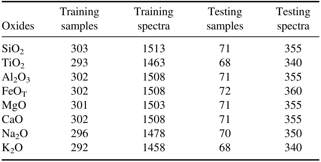
Table 1.The number of samples and spectra of training set and testing set used in this study.

The spectra used in this paper have already been preprocessed.The pre-process included subtraction of non-laser dark spectrum,removal of noise,reduction of continuum spectrum,wavelength calibration,instrument response measurement and distance correction.More details about the preprocess can be found in[21].Besides,in order to reduce the order of magnitude,the min-max normalization is used to normalize spectra data,which is the only pre-process performed in this paper.The conversion function is as follows:

where x is one of the observations,xminis the smallest observation,xmaxis the largest observation and z is the new observation.

3.Methodology

3.1.Convolutional neural network

CNN is a deep learning method widely used for target classification,target detection,and target recognition[22-24].In recent years,CNN has been successfully utilized for the LIBS quantification due to its outstanding capability of feature extraction[19,25].CNN has two important characteristics(sparse connectivity and shared weights)which can greatly reduce the number of the parameters that the network needs to be compared to ANN.A CNN model generally consists of an input layer,convolutional layers,excitation layers,pooling layers,fully-connected layers and an output layer.The convolution kernel used for feature extraction is a core part of the CNN model.Convolutional kernels of different sizes can extract features of different levels and the stacked convolutional layers can extract features of higher abstraction.For one-dimensional spectral data,we used 1×n convolutions.There are activation functions in the excitation layer,which act on the outputs of the convolutional layers.The activation functions in the excitation layers make the CNN model have the capability of nonlinearly mapping.The CNN model with an activation function can better solve more complex problems.The hyperbolic tangent(tanh)function,the rectified linear unit(ReLU)function,the linear function and the Sigmoid function are used as activation functions to train the CNN models in this paper respectively.The forms of the tanh function,the ReLU function,the linear function and the Sigmoid function are:

where x is one of the outputs of the convolutional layers.

In addition,to improve the performance of the deep neural network,the Inception V2 architecture that can increase the depth and width of the network was used to construct the CNN regression model in this study.The Inception V2 architecture was proposed by Ioffe et al[26]in 2015.The Inception V2 architecture used in this paper is shown in figure 2.The four paratactic branches of the Inception V2 architecture have different functions.All the 1×1 convolutions of the four branches can reduce the number of the feature maps.The function of the 1×3 convolutions of the second branch is feature extracting.Two 1×3 convolutions in sequential order in the Inception V2 architecture(the third branch)are used to replace the 1×5 convolutions in Inception V1 architecture,which can provide more nonlinearly mapping and reduce the number of the parameters of the network.The role of the max pooling of the forth branch is improving the receptive field,reducing the dimension of the feature maps and increasing translationinvariant to some extent.However,because we used the max pooling with a stride of 1,the dimension of the feature maps did not reduce.In essence,the workings of the Inception V2 architecture can be described in the following two steps:(1)obtaining feature maps of different levels from four branches;(2)integrating feature maps of different levels together.

3.2.Experiments

3.2.1.Constructing CNN regression models.The CNN model we constructed for one-dimensional spectral data is shown in figure 3.There are three convolutional layers(Conv1,Conv2 and Conv3)behind the input layer,which can capture spectral details.The Inception V2 architecture behind the convolutional layers can further extract spectral features of different levels and the concatenation layer can integrate features of different levels together.The flatten layer can transform multi-dimensional data into one-dimensional data,which is the transition from a convolutional layer to a fully-connected layer.The settings of each convolutional kernel(or max pooling)are shown in table 2.

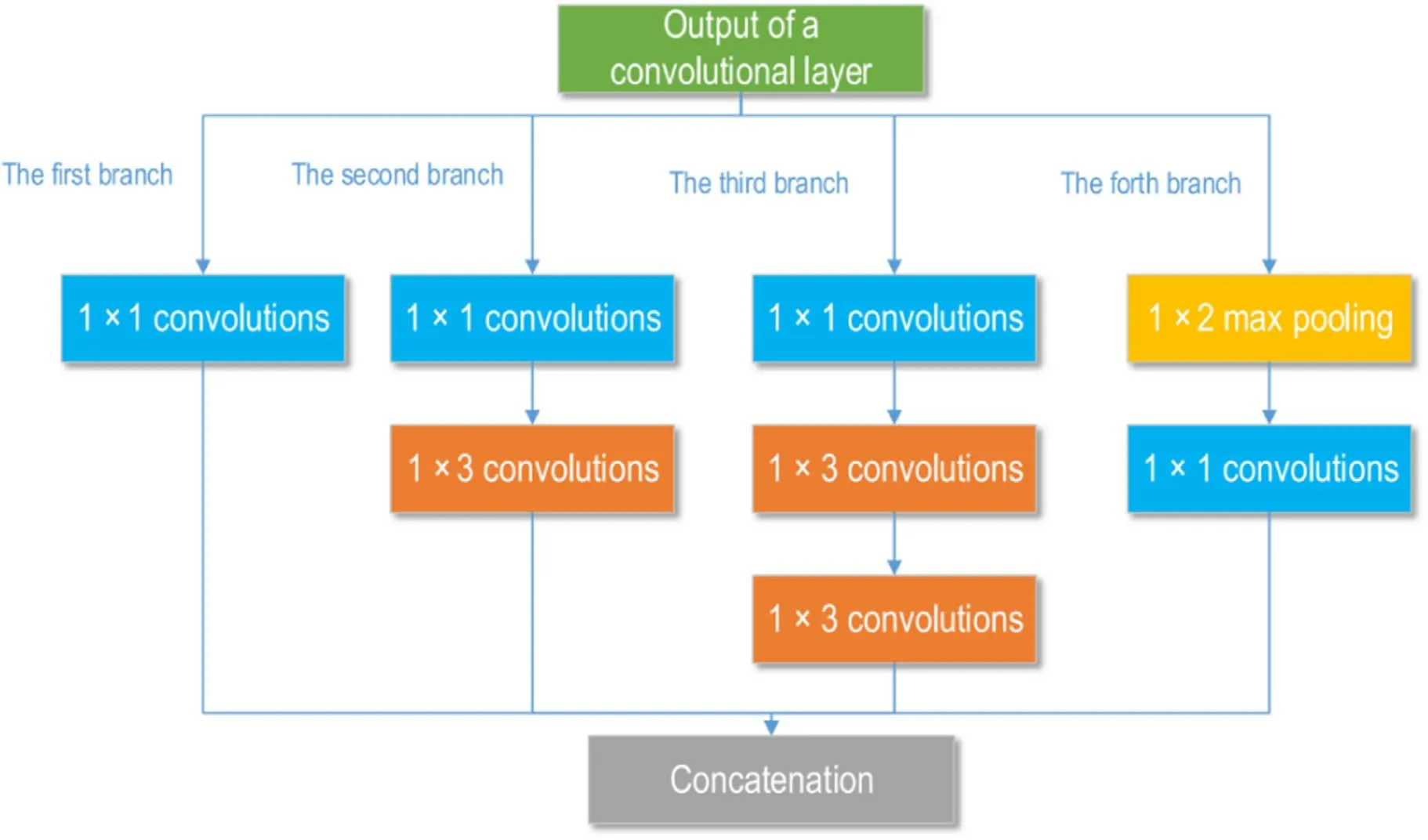
Figure 2.The architecture of the Inception V2.

Figure 3.The structure of the proposed model.

We used the trial-and-error method to choose a better activation function for the CNN regression model.In our study,we compared the effects of four different activation functions(the tanh function,the ReLU function,the linear function and the Sigmoid function)on the regression model.Before comparison,we paired each activation function with an appropriate weight initialization method.The weight initialization that sets a corresponding initial value for each weight is an important part of the CNN model.A good initialization method can accelerate the process of training to converge and is more likely to find a better solution.Conversely,a bad initialization method may cause problems in the process of gradient propagation.Hence,choosing a suitable initialization method is essential for training a network.Two initialization methods namely ‘Xavier’ and‘He_normal’which are often utilized in neural networks were used in this study.The basic idea of the‘Xavier’initialization is to make the output and input of each network’s layer have a normal distribution and similar variance to avoid the output becoming zero.For the ReLU function,if the input value is less than zero,the output would be zero,which affects the output distribution.Hence,the‘He_normal’initialization was proposed to solve the above phenomenon.Since the ‘Xavier’initialization is helpful for the tanh function,we used the‘Xavier’ initialization for the CNN model with the tanh function(t-model).Being beneficial to the ReLU function,the‘He_normal’ initialization was selected for the CNN model with the ReLU function(r-model)[27,28].For the model with the linear function(l-model)and the model with the Sigmoid function(s-model),we used the ‘He_normal’initialization.When we compared the performance of four activation functions,the other parameters of the CNN model are exactly the same.

After choosing a suitable activation function,we explored the effects of the optimization methods on the regression models.In the process of BP,the gradient descent optimization algorithms are often used to update the weights of the convolutional kernel.A good optimization method can make the model converge quickly and get a better solution.An inappropriate optimization method may make the model unable to converge or have a large prediction error.Besides,the initial learning rate of the optimization method is also an important part of training a neural network.In our study,we used the stochastic gradient descent(SGD)optimization[29]and the Adam optimization[30]to train the CNN model we built,respectively.SGD that updates the weights by a gradient from a stochastic spectrum in each epoch is one of the most commonly used algorithms.Adam which is an adaptive optimization algorithm has been a popular optimization method for a neural network in recent years.For these two optimization methods,three different initial learning rates(0.01,0.001 and 0.0005)were used to train the CNN model,respectively.

Being an essential part of the CNN model,the loss function provides errors for error back propagation algorithms and concerns the performance of the regression model.The mean square error(MSE)loss function was thus selected for training the CNN model.To improve training speed and reduce overfitting,a batch normalization layer was placed behind the full-connected layer.A mechanism called ‘early stopping’ was used to stop the training model to avoid overfitting.

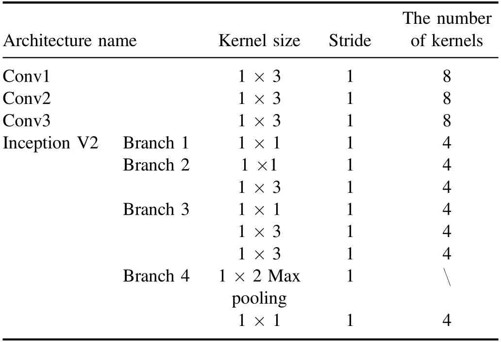
Table 2.The settings of each convolutional kernel(or max pooling)used in the CNN regression model.

Table 3.Optimized C and γ of the SVR model for all oxides.

3.2.2.Comparison among the performance of the CNN model,the SVR model and the PLSR model.After choosing a better activation function,a suitable optimization method and an initial learning rate for the CNN model,the comparison among the performance of the CNN model,the SVR model and the PLSR model was performed.In this section,the process of parameter optimization of the SVR model and the PLSR model was described.

国内外文献主要聚焦数字化变革给传统出版业带来的冲击，例如，信息技术（如“云出版”）、管理创新（如编辑流程重构、“融”出版、众筹出版等）和政策扶持等对传统出版业的经营理念、营销渠道和产业分工合作等产生重要影响。然而，现有文献更多关注大型出版集团的信息化变革与应对，忽略了对中小出版企业的转型升级研究。位于产业“金字塔”底部的中小出版企业转型升级到底有哪些路径可走？需要理论界进一步开展研究。本文基于“新三板”挂牌新闻和出版企业数据分析，揭示中小出版企业转型升级的实践，弥补现有文献对出版企业实践分析的不足，对国家政策实施和企业经营具有现实意义。

To train an SVR model,two essential parameters(C and γ)need to be optimized,which determine the performance of the regression models.As a key factor for the establishment of the hyperplane,C represents the fault-tolerance.γ is the vital parameter of the radial basis function which maps the spectra into a higher dimensional linear separable space[31].Furthermore,the number of support vector influences the speed of model training.The solution for best choosing the two key parameters was to utilize the grid optimization algorithm coupled with a three-fold cross validation(CV)in the training set.C and γ under the minimum root mean square error of cross validation(RMSECV)were chosen as the final parameters of the SVR models.More details about the SVR model can be found in table 3.PLSR extracts the principal components(PCs)from two matrices(i.e.samples(X)and the corresponding labels(Y))respectively and then models the relationship between two matrices.The number of PCs is a key parameter of PLSR,which concerns the prediction capability of the PLSR model[32].In this paper,we optimized the number of PCs by a three-fold CV in training data.Table 4 shows the best number of PCs for all oxides.

The CNN models in this research were done in Python using Keras.The SVR model and the PLSR model were completed using MATLAB 2016.The parameters-optimized process of the SVR model and the PLSR model was implemented on the MATLAB 2016.

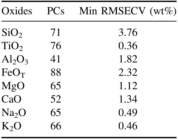
Table 4.The best number of PCs of the PLSR model for all oxides.

3.3.Model evaluation

Since the initial weights of the CNN model are not fixed values,there are little differences among the performance of the models trained at different times.Therefore,in this study,we repeated the process of training the CNN model ten times,and took the average value of ten root mean square errors of predicted concentrations(RMSEP)as one of the indicators to evaluate the prediction capability of the regression models.Besides,standard deviation(SD)of ten RMSEPs was used to evaluate the stability of the model.The forms of RMSEP and SD are described in the following equations:

where yi,actualis the actual value of ith sample,yi,predictedis the predicted value of ith sample,N is the number of testing spectra,RMSEPjis the jth RMSEP,RMSEPaverageis the average value of all RMSEPs and M is the number of RMSEPs.

4.Results

4.1.Effects of four activation functions on the CNN model

In order to find a suitable activation function for the CNN model,we compared the performance of the t-model,the r-model,the l-model and the s-model.There are some predetermined parameters in these CNN models:the SGD optimization,the initial learning rate=0.0005 and the batch size=256.Table 5 shows the performance of these CNN models for all oxides.For SiO2,TiO2,Al2O3,MgO and K2O,the t-model has the best performance when compared to the other three CNN models.For FeOTand CaO,the t-model has the second best performance which also is an acceptable result.For Na2O,the t-model obtains an average RMSEP of 0.44 wt%,which is almost the same as that of the r-model(average RMSEP=0.43 wt%).Overall,for each oxide,the t-model has a satisfactory performance.

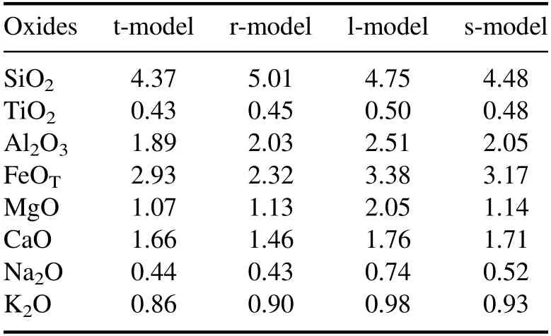
Table 5.The average RMSEP(wt%)of the t-model,the r-model,the l-model and the s-model for all oxides.

Table 6.The SD(wt%)of ten RMSEPs of the t-model,the r-model,the l-model and the s-model for all oxides.

In addition,we compared the SDs to study the stability of the CNN models.Table 6 exhibits the SDs of the abovementioned four models.The SD of l-model’s ten RMSEPs is lower than the SD of the other three CNN model’s ten RMSEPs for all oxides except Na2O.Compared with the other three models,for all oxides except SiO2and CaO,the s-model has the second best performance in terms of SD.Although the stability of the l-model and the s-model is better than that of the t-model and the r-model,their prediction error is greater than the prediction error of the t-model and the r-model for all oxides except SiO2.Notice here our priority is the prediction accuracy,and the SDs of the t-model and the r-model are acceptable for all oxides.For TiO2,Al2O3,MgO,CaO and K2O,the SD of the t-model’s ten RMSEPs is lower than the SD of r-model’s ten RMSEPs.For SiO2,FeOTand Na2O,although the SD of the t-model’s ten RMSEPs is bigger than the SD of the r-model’s ten RMSEPs,the difference value between them is very small.Based on the above analysis,it is obvious that the tanh function is more helpful than the ReLU function,the linear function and the Sigmoid function for constructing CNN models on the ChemCam calibration data.

4.2.Choosing a suitable optimization method and an initial learning rate for the CNN model

Before exploring the effects of different optimization methods on the performance of the CNN model,we predetermined the activation function:the tanh function.For the SGD optimization and the Adam optimization,three different initial learning rates were used to train the CNN model,respectively.Table 7 exhibits the average RMSEPs of the CNN models with different optimization methods and initial learning rates.For SiO2,Al2O3,FeOTand MgO,the model with the SGD optimization and the initial learning rate=0.0005 obtains the best performance compared with the other CNN models.For Na2O and K2O,the model with the SGD optimization and the initial learning rate=0.0005 has the second best performance which is not much different from the best model.For TiO2,the RMSEP of the model with the SGD optimization and the initial learning rate=0.0005 is 0.43 wt%,which is an acceptable result compared to the other models.For CaO,the model with the SGD optimization and the initial learning rate=0.0005 provides a bad RMSEP when compared to the other three CNN models with the Adam optimization.The reason why the CNN model with the SGD optimization and the initial learning rate=0.0005 did not find the global optimal solution may be the initial learning rate=0.0005 is not suitable for training the CNN model for CaO.For the SGD optimization,the model with the initial learning rate=0.0005 is slightly better than the model with the initial learning rate=0.001 for all oxides except Na2O.However,the model with the SGD optimization and the initial learning rate=0.01 did not converge for some oxides(SiO2,Al2O3,FeOT,MgO,CaO and K2O),which illustrates that a proper initial learning rate is important for the SGD optimization.For the Adam optimization,because of the feature of adaptive adjustment of the learning rate,several CNN models have similar performance for all oxides except FeOTand MgO.On the whole,the model with the SGD optimization and the initial learning rate=0.0005 models still has advantages over the other models.

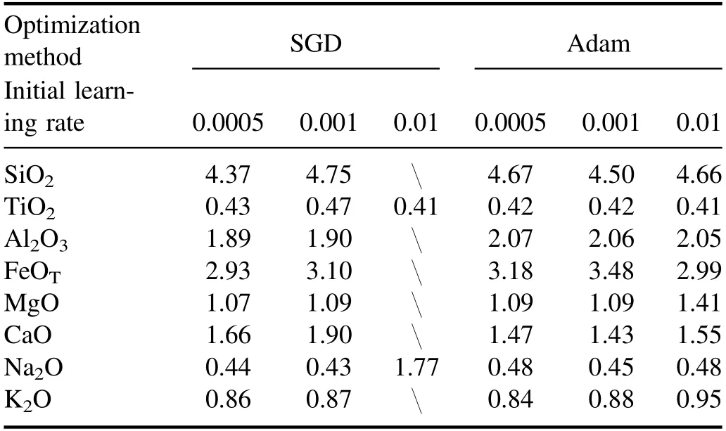
Table 7.The average RMSEP(wt%)of the CNN models for all oxides(‘’ represents the model did not converge).

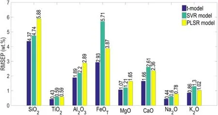
Figure 4.The performance of the t-model,the SVR model and the PLSR model.

Table 8 shows the SD of each CNN model’s ten RMSEPs for all oxides.For the SGD optimization,the SD of the model with the initial learning rate=0.0005 is less than or equal to those of the other two models for all oxides except Al2O3.For the Adam optimization,the SD of the model with the initial learning rate=0.0005 is less than or equal to those of the other two models for all oxides except TiO2and CaO.From an overall perspective,the SD of the model with the SGD optimization and the initial learning rate=0.0005 is similar to the SD of the model with the Adam optimization and the initial learning rate=0.0005 for all oxides except Al2O3and FeOT.Therefore,the model with the SGD optimization and the initial learning rate=0.0005 has satisfactory stability.

Considering the prediction accuracy and the stability,we think the SGD optimization and the initial learning rate=0.0005 are the best choice for the CNN model we constructed.Compared to setting a suitable set of parameters for the CNN model of each oxide,the model with unified parameters for all oxides is efficient and concise.

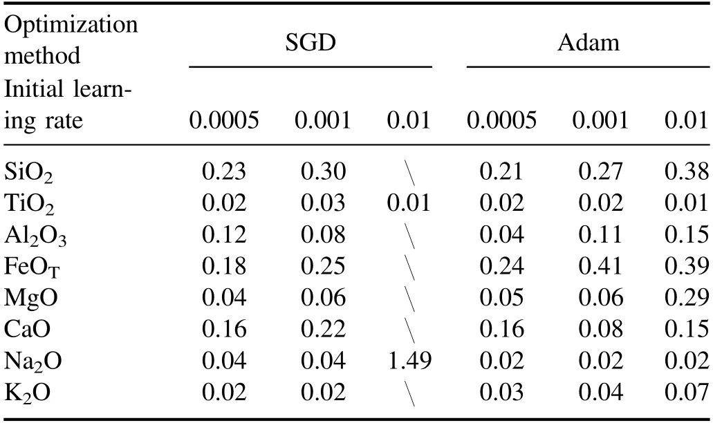
Table 8.The SD(wt%)of ten RMSEPs of the CNN models for all oxides(‘’ represents the model did not converge).

4.3.Comparison of the results obtained by the t-model,the SVR model and the PLSR model

The t-model,the optimization of which is the SGD optimization and the initial learning rate of which is 0.0005,was chosen as the final CNN regression model in this study.To prove that the t-model has a better prediction capability than the SVR model and the PLSR model,we compared the performance of these three models.The performance of these three models is shown in figure 4.For SiO2,the SVR model obtains a RMSEP of 4.74 wt% which is smaller than the PLSR model’s RMSEP and bigger than the t-model’s average RMSEP.For TiO2,the RMSEP of the SVR model is equal to that of the PLSR model and is bigger than the average RMSEP of the t-model.For Al2O3,MgO and Na2O,the SVR model’s RMSEP is smaller than the PLSR model’s RMSEP and is bigger than the t-model’s average RMSEP.For FeOT,the average RMSEP of the t-model is lower than the RMSEPs of the SVR model and the PLSR model.For CaO,the RMSEP of the SVR model is 2.61 wt% and the RMSEP of the PLSR model is 2.36 wt%,which are all bigger than the average RMSEP of the t-model.For K2O,the t-model provides the best performance with an average RMSEP of 0.86 wt%and the second best model is the SVR model.In the mass,the t-model’s average RMSEP is much less than the other two models’ RMSEPs for all oxides.It is obvious that the t-model can effectively develop the prediction accuracy when compared to the SVR model and the PLSR model.

Figure 5.For SiO2 and TiO2,the plots of the actual values versus the predicted values(red points:the best t-model,blue points:the SVR model,black points:the PLSR model).

Figure 6.For Al2O3 and FeOT,the plots of the actual values versus the predicted values(red points:the best t-model,blue points:the SVR model,black points:the PLSR model).

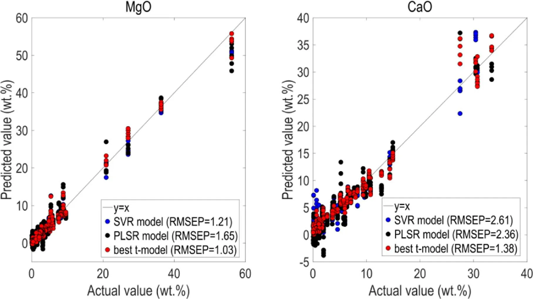
Figure 7.For MgO and CaO,the plots of the actual values versus the predicted values(red points:the best t-model,blue points:the SVR model,black points:the PLSR model).

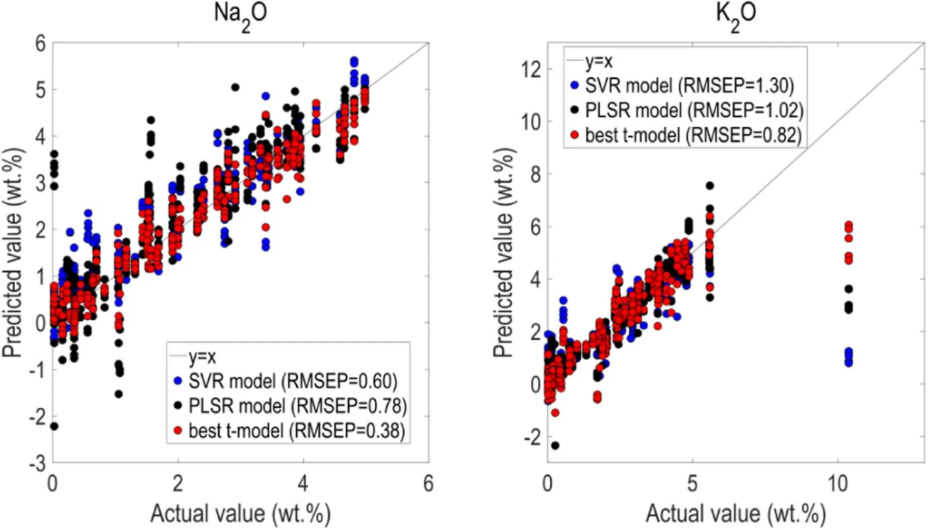
Figure 8.For Na2O and K2O,the plots of the actual values versus the predicted values(red points:the best t-model,blue points:the SVR model,black points:the PLSR model).

We used the average value of ten RMSEPs of the t-model to evaluate the prediction capability of the t-model.However,if the t-model actually gets used,we need to use the best t-model among ten models for determining the components of the targets.Figures 5-8 show the plots of the actual concentrations against the predicted concentrations of testing samples for the best t-model(among ten t-models),the SVR model and the PLSR model.The distance of the point to the y=x line presents the loss of the predicted value.The shorter the distance is,the smaller the loss is,and the more accurate the predicted value is.For eight oxides,we can visually find the red points that belong to the t-model are closer to the y=x line than the blue points(the SVR model)and the black points(the PLSR model).It is no doubt that the t-model is superior to the SVR model and the PLSR model.We owed these phenomena to the powerful feature extraction capability of the CNN algorithm.Different convolution kernels can extract features of different levels and the Inception V2 architecture can integrate features of different levels together,which provides more spectral details.In addition,features of higher and lower abstraction can effectively reduce the chemical matrix effects.These advantages contribute to the CNN model with wonderful performance when applied for the LIBS quantification of the one-dimensional ChemCam spectral data.

5.Conclusion

In this study,we constructed a CNN regression model for the LIBS quantification of the one-dimensional ChemCam spectral data.In the first place,in order to choose a suitable activation function for the CNN regression model,we compared the effects of four activation functions on the performance of deep neural networks.The results show that the t-model outperforms the other three models(the r-model,the l-model and the s-model).Next,we explored the effects of optimization methods on the CNN models.By comparison,the model with the SGD optimization and the initial learning rate=0.0005 that has better prediction accuracy and satisfactory stability was chosen as the final CNN regression model.Finally,we compared the performance of the t-model,the SVR model and the PLSR model.The results show that the average RMSEP of the t-model is much smaller than the RMSEPs of the SVR model and the PLSR model.In conclusion,the t-model significantly improved the capability of predicting the elementary composition of diverse targets when used for the ChemCam calibration data.The excellent performance of the CNN regression model illustrates that CNN can effectively overcome the chemical matrix effects and can be successfully applied for the LIBS quantification of the one-dimensional ChemCam spectral data.

In the first Mars Global remote sensing and regional survey mission of China,MarsCoDe based on LIBS will be used to explore Mars material composition.The CNN model proposed in this study can be served for the LIBS quantification of MarsCoDe.Improving the prediction capability of the regression model is still an important issue for the future exploration of Mars materials.Therefore,more research is needed to be conducted in the future to refine and improve the regression models used for the quantitative analysis of LIBS.

Acknowledgments

This work is supported by the Pre-research project on Civil Aerospace Technologies(No.D020102)funded by China National Space Administration(CNSA).We also thank the funding from National Natural Science Foundation of China(Nos.U1931211 and 41573056),the Natural Science Foundation of Shandong Province(No.ZR2019MD008)and the Major Research Project of Shandong Province(No.GG201809130208).