Reconstruction of Probability Density Function for Gamma Distribution

FANJinwei(范晋伟)，LIZhongsheng(李中生)，TIANBin(田斌)

1 Beijing Key Laboratory of Advanced Manufacturing Technology, Beijing University of Technology, Beijing 100124, China2 Neijiang Jinhong Crankshaft Co., Ltd., Neijiang 641000, China

Abstract: The probability distributions of small sample data are difficult to determine, while a large proportion of samples occur in the early failure period, so it is particularly important to make full use of these data in the statistical analysis. Based on gamma distribution, four methods of probability density function (PDF) reconstruction with early failure data are proposed, and then the mean time between failures (MTBF) evaluation expressions are concluded from the reconstructed PDFs. Both theory analysis and an example show that method 2 is the best evaluation method in dealing with early-failure-small-sample data. The reconstruction methods of PDF also have certain guiding significance for other distribution types.

Key words: small sample; probability density function (PDF); gamma distribution; early failure; mean time between failures (MTBF)

Introduction

With the rapid development of Internet of things and cloud computing in recent years, big data become more and more important. However, the small sample issue is also necessary in engineering practice. In particular, it is a more common situation, such as for a weapon system, or a system operating in completely different environments, or a security issue, or an expensive test process[1]. Therefore, the statistical technology based on small samples is still essential. With the diversified development of society, the small sample issue is more significant than the big data issue in many cases[2].

Some scholars have already done significant research on statistical technology based on small samples. For instance, to get a more accurate confidence interval, Fulton and Abernethy[1]developed the justified likelihood function method based on small sample data. To study small sample issues, Lam and Spelt[3]utilized the modified likelihood ratio (LR) test where the Fulton factor was used to remove the majority of the bias. Fulton and Abernethy[1]presented the results of Monte Carlo simulation to estimate the Type II error occurrence on the Weibull distribution. Based on zero-failure data during the reliability test, Jiangetal.[4]proposed a modified maximum likelihood estimate (MMLE) to estimate the parameters of Weibull distribution. Then, the shrinkage preliminary test estimator (SPTE) was constructed by incorporating the MMLE and the prior probability estimate from a similar product. Finally, the effectiveness of the proposed SPTE was demonstrated by an example.

The above researches indicated that, the optimized parameter estimators of probability density function (PDF) were obtained, through Bayesian method or enlarging sample size (such as Bootstrap[5], Support Vector Machine[6], Neural Network, and fuzzy mathematics theory[7]). Then the mathematical expectation of the lifetime was determined through numerical integration, and thus the reliability indexes were obtained. However, each extending-sample-size method has a specific application scope. Therefore, the analysis results of each method have limitations. Moreover, data mining of small samples for the complex repairable systems are important[8].

In addition, most of the small sample failure data come from the early failure period of the life cycle. In fact, these failures caused by abnormal reasons or quality problems can be effectively controlled by the process improvement[9]. Furthermore, the early failure rates of some equipments are even bigger than one half of the total rate in the life cycle[10]. Therefore, it is necessary to develop an effective evaluation algorithm, by fully utilizing these failure data in the early failure period.

The failure rate, also called as the rate of occurrence of failures, normally conforms to the bathtub-shaped curve. That is, when the product is put into use, the failure rate is higher. Then the failure rate is gradually reduced and tends to be gentle in the normal operating period. Most of the existing studies are based on the normal operating period with a flat failure curve. However the study based on the early failure period is less.

This paper presents some mathematical methods to reconstruct PDF involving the early failure data, inspired by Mnatsakanov[11]and Yuetal.[12]The new PDF will then replace the original one and be used in statistical and reliability studies.

1 Background Review

As the foundation of study for the probability assessment and life cycle analysis, the failure rateh(t), is defined as the number of failures per unit time per number of non-failed products remaining at timet[13]. In general,h(t) branches out into three categories: monotonic failure rates; bathtub-shaped failure rates (h(t) has a bathtub or a U shape); and generalized bathtub-shaped failure rates[14]. Because most products have non-monotonic failure rate functions, the bathtub-shaped life distribution is used widely, which can be divided into three periods: the early failure period, the normal operating period and the wear-out period[15].

A popular life distribution—gamma distribution, which can provide a good fitting to many sets of failure data[16-17], is chosen for study in this paper. The PDF of a two-parameter gamma distribution is given as[13]

(1)

where Γ(η) is the gamma function,tis the operating time andt≥0,ηis the shape parameter, andλis the scale parameter.

The cumulative distribution function (CDF) of a two-parameter gamma distribution is expressed in terms of the definition.

(2)

wheret≥0, then mean time between failures (MTBF) expression are obtained accordingly.

(3)

(4)

(5)

whereR(t) is the reliability function andt≥0,h(t) is the failure rate function, andMis the MTBF. When the parameters of a gamma distribution are fixed, the alternative MTBF expression is

(6)

The reconstructed PDFs will be discussed based on Eqs. (1)-(6).

2 Reconstruction Study of PDF

A typical failure rate curve of a two-parameter gamma distribution is plotted as shown in Fig.1, and also known as the bathtub-shaped curve (partial). The knee point of the bathtub-shaped curve denotes that the curve is divided into two parts. That is, the early failure period is defined as the period from zero to timeτ1, which illustrates that the failure rate is very high at the beginning of use, but it decreases rapidly with the increase of working hours. The normal operating period is defined as the period from timeτ1, which shows that the failure rate is lower and stable in this period. Furthermore, the cumulative failure rate during the early failure period can be calculated.

In Eq. (4), the early cumulative failure rate shall be transformed from the failure rate functionh(t) to the PDF. First, the early cumulative failure rate, also named early failure proportionsh(τ1), can be calculated through dividing the early failures withinτ1by all failures. Next leth(τ1) equal the early cumulative failure rate of PDF,F(t1). Then, the assumed dividing pointt1of PDF, can be obtained according to Eq. (2). That is, the cumulative early failure rate on the bathtub-shaped curve (from zero toτ1) is transplanted to the PDF curve (from zero tot1). The transplantation can be expressed by

(7)

The datum time-point (T1) is expected for statistical study, which is assumed at the inchoate stage in the normal operating period as shown in Fig. 1. Thus, four PDF reconstructing methods are discussed.

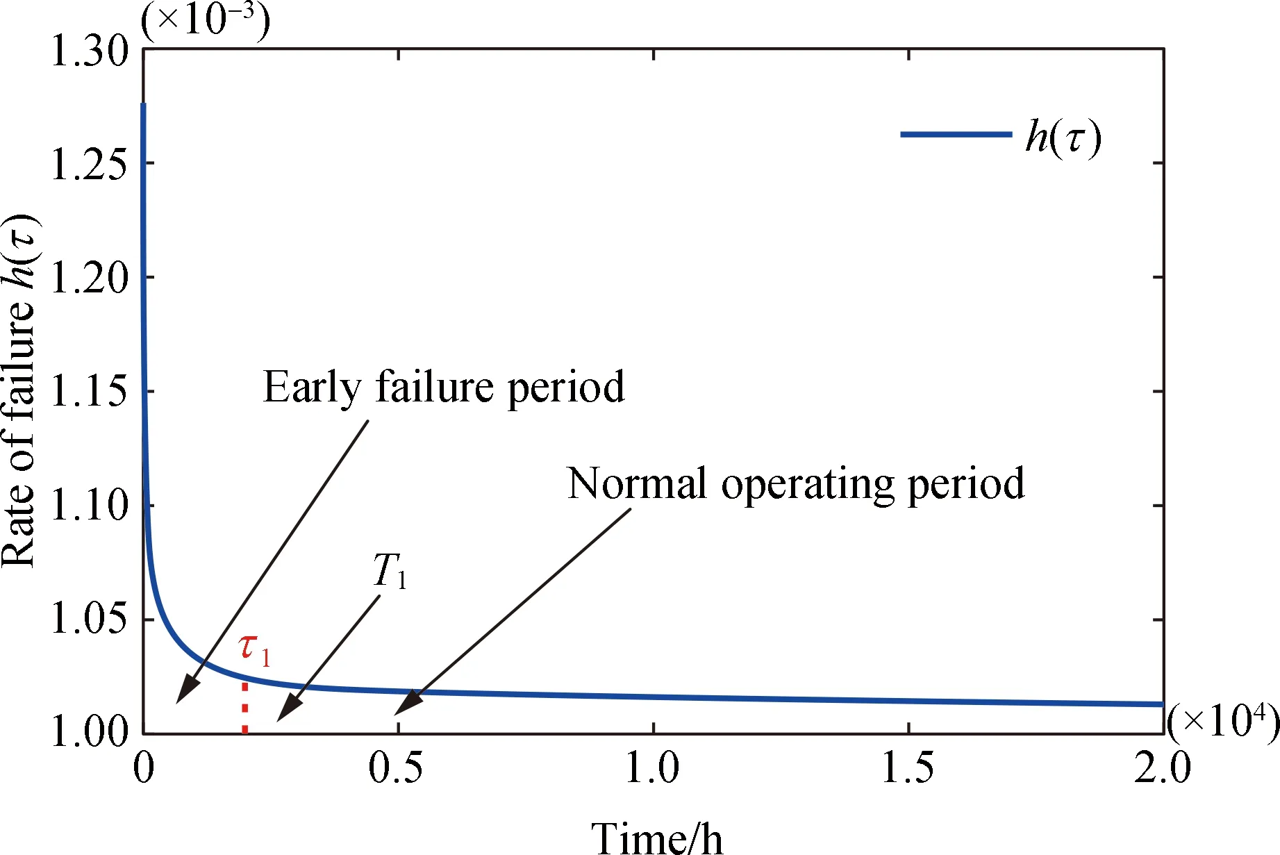
Fig. 1 Rate of failure

Method1The early cumulative failureF(t1)0will be deleted fromF(t)0. Then it is reallocated to the whole life-cycle equally. It is proved that the whole cumulative failure rate equals 1. So, the compensation expression is defined as

,

(8)

whereTis the test duration.

The new PDF is obtained as

(9)

The details off(t)1andf(t)0are shown in Fig. 2.

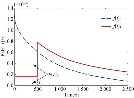
Fig. 2 Comparison of f(t)1 and f(t)0

Thus, the deviation rateσ1is got.

(10)

Method2The early cumulative failure,F(t1)0, is also deleted from the initial PDFF(t)0. Then it is redistributed to the whole life cycle in terms off(t)0. It is also proved that the whole cumulative failure rate equals 1. Thus, the compensation expression is defined as

(11)

The new PDF is expressed as

(12)

The details off(t)2andf(t)0are shown in Fig. 3.

The deviation rateσ2is calculated as

(13)

According to Eqs. (2)- (3), (11) and (12), the CDFF(t)2is obtained.

-R(t)0F(t1)0+F(t)0, (t>t1).

(14)

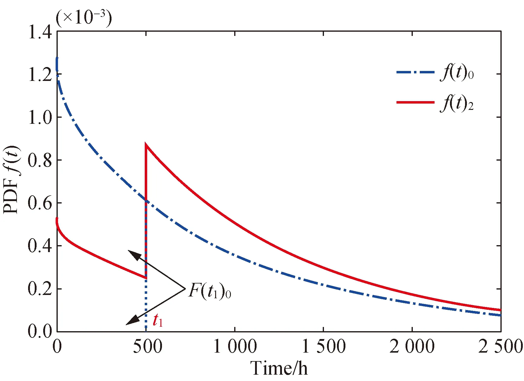
Fig. 3 Comparison of f(t)2 and f(t)0

Method3The start time-point of the new reconstructed PDFf(t)3, is set for parallel moving backwardt1hours. That is,f(t)3is supposed to perform fromt1to the end of the lifetime. While the early cumulative failure,F(t1)0, is removed from the original PDFf(t)0. Then it is redistributed to the new PDFf(t)3according tof(t)0(from zero to the whole life cycle). Thus, the relative expressions are obtained.

The compensation is

(15)

The new PDF is

f(t)3=δ(t1)3+f(t+t1)0.

(16)

It is proved that the cumulative failure rate from zero to infinity of the new PDFf(t)3, equals 1 below.

(17)

The details off(t)3andf(t)0are shown in Fig. 4. The deviation rateσ3is obtained as

exp(-λt1)+F(t1)0-1,(t→∞).

(18)

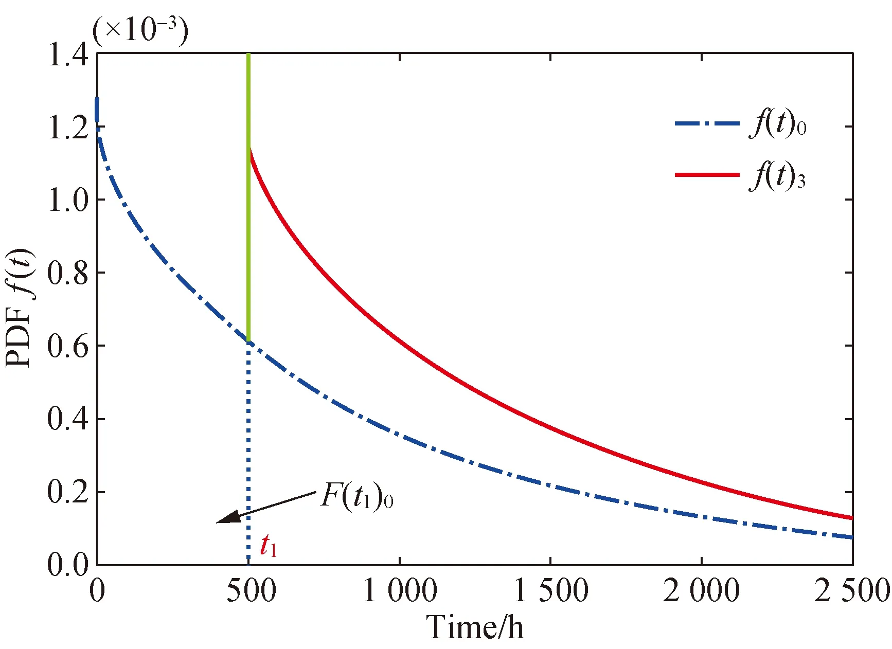
Fig. 4 Comparison of f(t)3 and f(t)0

Method4The start time-point of the new PDFf(t)4, is similarly set for parallel moving backwardt1hours. That is,f(t)4is also supposed to perform fromt1to the end of lifetime. While the early cumulative failure,F(t1)0, is deleted from the initial PDFf(t)0,F(t1)0is then reallocated tof(t)4, in accordance withf(t+t1)0(fromt1to the whole life cycle). Thus, the relative expressions are obtained as well.

The compensation is

F(t1)0f(t+t1)0.

(19)

The new PDF is

f(t)4=δ(t1)4+f(t+t1)0=

(1+F(t1)0)f(t+t1)0.

(20)

It is proved that, the cumulative failure rate from zero to infinity of the new PDFf(t)4does not equal 1.

(1+F(t1)0)(1-F(t1)0)=

1-F2(t1)0.

(21)

The details off(t)4andf(t)0are shown in Fig. 5.

Fig. 5 Comparison of f(t)4 and f(t)0

In summary, regarding method 1, when the running time tends to infinity, its deviation rate tends to infinity, so it is not suitable for practical application. For method 2 and method 3, the cumulative failure rates all equal 1. For method 4, the cumulative failure rate does not equal 1. Moreover, method 2 shall express the probability density at any time in the life cycle, while method 3 can only describe the probability density in the normal operating period. Therefore, the PDF constructed by method 2 is theoretically more reasonable and comprehensive. Hereby, four reconstructed PDFs with three detailed expressions have been discussed. The application will be discussed in section 3.

3 Applications

3.1 MTBF assessment

According to the existing literature, MTBF is the most important indicator to describe the system reliability[2, 18]. Thus, the MTBF assessment expressions are deduced based on the reconstructed PDFs.

Inference1The new reconstructed PDFf(t)1doesn’t converge onf(t)0as time increased, which can be concluded according to Fig. 2 and Eq. (10). So,f(t)1is unsuitable for MTBF assessment. Moreover, the new PDFf(t)1is discontinuous at timet1.

Inference2The deviation rateσ2is a constant, ift1is fixed. Thus, the new reconstructed PDFf(t)2can be utilized for MTBF assessment. Here,f(t)2is used to describe the MTBF expression on behalf off(t)0.

According to Eqs. (3) and (5), the prediction expressions are obtained as

R(t)2=1-F(t)2=

1-(-R(t)0F(t1)0+F(t)0)=

(1+F(t1)0)R(t)0,

(22)

(1+F(t1)0)M0,

(23)

whereM0is the MTBF calculated byf(t)0,t>t1.

Inference3The deviation rateσ3is a constant， ift1and the parameters of gamma distribution are fixed, sof(t)3also can be utilized for MTBF prediction. The new reconstructed PDFf(t)3is used to express the MTBF on behalf off(t)0. According to Eqs. (5), (15)-(16), the prediction expression,M3is obtained.

(24)

Inference4The total residual valueν4, which includesF2(t1)0, could be obtained, if the supposed time-pointT1for MTBF assessment is fixed.

(25)

As a result, the amended assessment expression can be expressed by addingν4*T1. In addition, the residual value (rate)F2(t1)0should be involved in the MTBF expression.

(26)

3.2 An illustrative example

As shown in Table 1, failure data used here were compiled from the development phases of three CNC grinders in a factory. The test duration for each CNC grinder wasT=4 500 h. The total number of failures was 12, and four failures were found for each grinder.

Table 1 Failure data of three CNC grinders

Previous studies have shown that the life distributions of this type of grinders are approximately subject to gamma distribution. After parameters estimation by maximum likelihood estimate (MLE), the PDF on the basis of the 12 failures was fixed as

(27)

which meets gamma distribution withη=0.963 andλ=1/989.

According to Eq. (6),M0=952.4 h was obtained, which ignored the impact of the data occurred in the early failure period. In contrast, the proposed prediction methods will be discussed as below.

Referring to Fig. 1, all of the 12 failures data were modeled by the dual gamma model[19-20], and the knee pointτ1was calculated as 2 000 h, under the goal of smooth connection of life curve between the early failure period and the normal operating period. That is, the early failure period was defined from zero to 2 000 h. In conclusion, totally 5 failures are found in the early failure period in Table 1.

In Eq.(7), the corresponding time-pointt1will be fixed. The actual early failure rateh(τ1), which is assigned from zero to 2 000 h, was calculated as 5/12= 41.67%. That is,F(t1)0was set to 41.67%. As a result, the corresponding time pointt1in CDF was calculated as 500 h approximately, according to Eqs. (2) and (27). Thus, the period from zero to 500 h in PDF was fixed as the early failure period.

Additionally, a criterion was finalized to appraise all of the proposed assessment methods[21]. Here, the real observed value of this type of CNC grinders was chosen as the standard. The data came from five CNC grinders, with the same configuration under three years, the total number of failures is 47. Thus, the real observed value is computed as

(28)

Three MTBF prediction results were listed in Table 2. To compare with the traditional methods, back propagation neural network (BPNN) was used to extend the original small samples, then the reliability evaluation was carried out according to the extended data. The MTBF value assessed by was about 1 000 h.

Table 2 Performance comparison of three methods and BPNN

As shown in Table 2, method 3 can’t reflect the influence of the early failure data. In contrast, method 2 and method 4 are appropriate for MTBF prediction, whose value is close to the actual observed value. The prediction value by BPNN is close to theM0.All of the prediction results are plotted in Fig. 6.

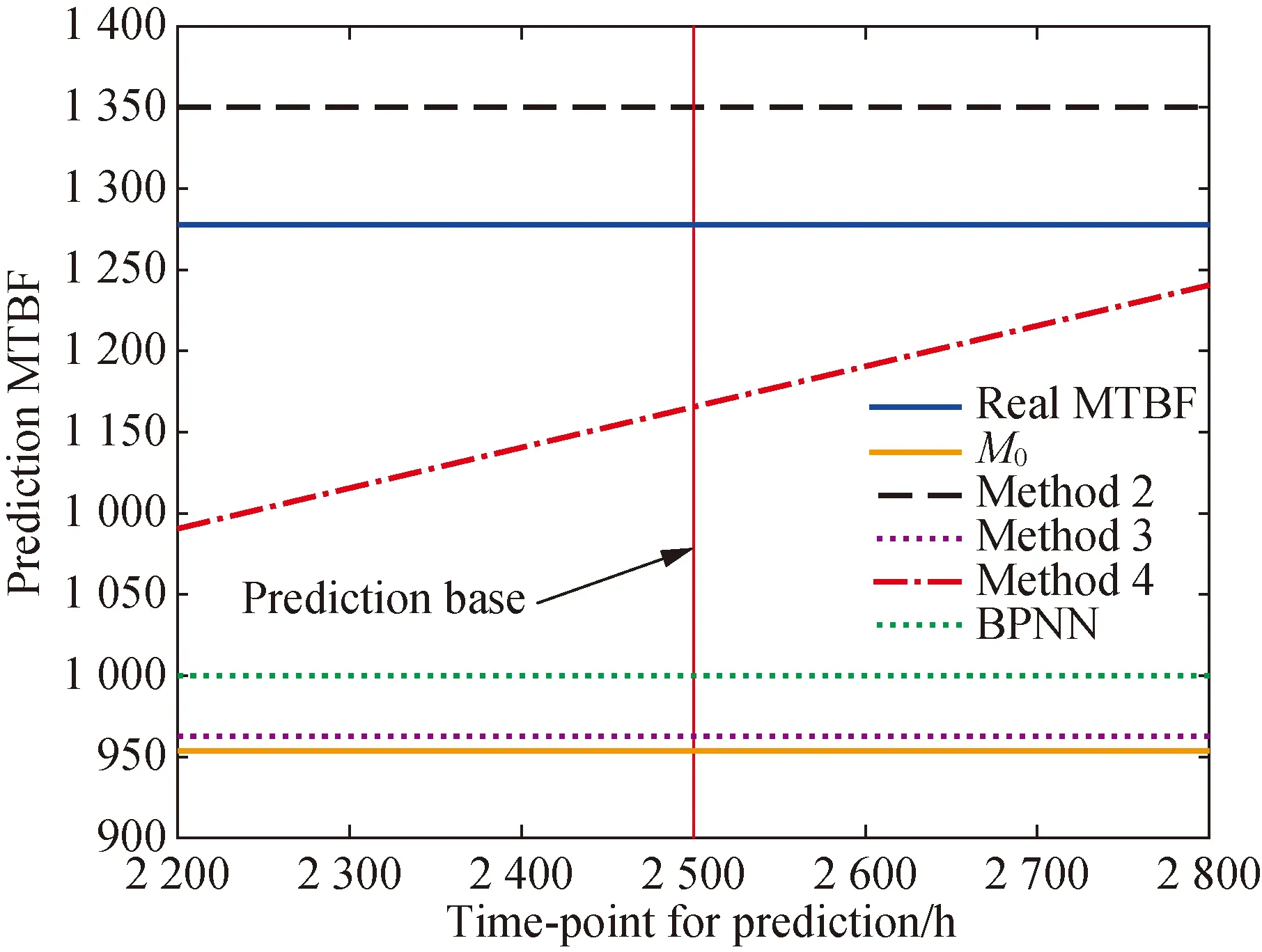
Fig. 6 Comparison of MTBF prediction for all methods

As shown in Fig. 6, the thin line indicates the prediction time base, which is defined as 2 500 h in the example. The solid lines indicate the real MTBF (upper) andM0(lower). The dashed line indicates the predicted MTBF via method 2. The lower dotted line indicates the predicted MTBF via method 3. The dashed-dotted line indicates the predicted MTBF via method 4. The upper dotted line indicates the predicted MTBF via BP neural network.

Furthermore, the prediction deviation rates of method 4 were calculated in a predefined interval, which was specified from 2 400 h to 2 600 h. The MTBF prediction value at 2 400 h was calculated as 1 147.4 h, and thus the deviation rate atT=2 400 h was calculated as: (1 277-1 147.4)/1 277=10.1%. Similarly, the MTBF prediction value at 2 600 h was calculated as 1 194.5 h. Hence the deviation rate atT=2 600 h was computed as (1 277-1 194.5)/1 277=6.5%. That is, the value of base time has a great influence on the prediction result. As a parallel result, for method 2, the prediction deviation rate was only (1 348-1 277)/1 277=5.6%. Thus, the method 2 is better than others.

4 Conclusions

It is an essential issue in probability and mathematical statistics to solve PDF based on the small samples, since PDFs contain almost all information of random variables. In many fields, for instance, engineering, economics, climatology and so on, all take the PDF as the basis to carry out the application research of practical problems.

By establishing the equivalent models of PDF, four reconstruction methods of PDF based on gamma distribution are proposed. The applications of reconstructed PDF are discussed through an example, which shows the method 2 has a good result on small samples, especially for the early failure data. Determining the knee point is the basis of dividing the life cycle, and its accuracy depends on the correctness and comprehensiveness of failure data. The defect of any statistical data will lead to the deviation of knee point, which will lead to the inaccuracy of failure period division and affect the credibility of the assessment results ultimately.

The reconstruction methods of PDF proposed in this paper also have certain guiding significance for other distribution types (exponential distribution, normal distribution, Weibull distribution,etc.). In addition, the reconstructed PDFs may be combined with artificial fault diagnosis technology to carry out early fault diagnosis research on industrial equipments.