FIO-ESM v2.0 Outputs for the CMIP6 Global Monsoons Model Intercomparison Project Experiments

Yajuan SONG, Xinfang LI, Ying BAO*, Zhenya SONG,Meng WEI, Qi SHU, and Xiaodan YANG

1First Institute of Oceanography, Ministry of Natural Resources, Qingdao 266061, China

2Laboratory for Regional Oceanography and Numerical Modeling, Qingdao National Pilot National Laboratory for Marine Science and Technology, Qingdao 266000, China

3Key Laboratory of Marine Science and Numerical Modeling, Ministry of Natural Resources, Qingdao 266061, China

ABSTRACT Three tiers of experiments in the Global Monsoons Model Intercomparison Project (GMMIP), one of the endorsed model intercomparison projects of phase 6 of the Coupled Model Intercomparison Project (CMIP6), are implemented by the First Institute of Oceanography Earth System Model version 2 (FIO-ESM v2.0), following the GMMIP protocols.Evaluation of global mean surface air temperature from 1870 to 2014 and climatological precipitation (1979-2014) in tier-1 shows that the atmosphere model of FIO-ESM v2.0 can reproduce the basic observed atmospheric features. In tier-2, the internal variability is captured by the coupled model, with the SST restoring to the model climatology plus the observed anomalies in the tropical Pacific and North Atlantic. Simulation of the Northern Hemisphere summer monsoon circulation is significantly improved by the SST restoration in the North Atlantic. In tier-3, five orographic perturbation experiments are conducted covering the period 1979-2014 by modifying the surface elevation or vertical heating in the prescribed region. In particular, the strength of the South Asian summer monsoon is reduced by removing the topography or thermal forcing above 500 m over the Asian continent. Monthly and daily simulated outputs of FIO-ESM v2.0 are provided through the Earth System Grid Federation (ESGF) node to contribute to a better understanding of the global monsoon system.

Key words: CMIP6, GMMIP, FIO-ESM v2.0, global monsoon

1. Background

The monsoon system, with its reversed wind vector in summer and winter, heralding the arrival of the rainy season, has significant influences on global climate (Trenberth et al., 2000; Wang, 2008). Anomalous monsoon can lead to natural disasters, characterized by extreme precipitation and temperature, and thus cause serious socioeconomic losses.The accurate simulation and prediction of the monsoon system is of broad societal concern (Webster et al., 1998).

Climate models are useful tools for studying the dynamic mechanisms and predicting changes of monsoon.The coupled atmosphere-ocean general circulation models(CGCMs) that participated in phase 5 of the Coupled Model Intercomparison Project (CMIP5) exhibit overall improvements in simulating climatological monsoon features, as compared with the CGCMs in CMIP3 (Sperber et al., 2013;Feng, 2014). However, the accuracy of simulations of intraseasonal variability, monsoon onset processes, extreme rainfall events, as well as the prediction of monsoon under global warming, remain as considerable scientific challenges for state-of-the-art CGCMs (Zhou et al., 2009; Cook et al., 2012; Sperber et al., 2013; Zou and Zhou, 2015). The inherent systematic biases in CGCMs, such as those caused by coarse resolution or an incomplete convection scheme(Anand et al., 2018), limit model ability to simulate monsoon well. Therefore, increasing the resolution and improving parameterization schemes are effective ways to consistently improve the simulation of monsoon precipitation and low-level circulation (Chen et al., 2010; Zhang et al., 2018).Moreover, numerous studies have shown that most models fail to capture the relations between monsoon and realistic climatic variabilities, such as El Niño-Southern Oscillation,the Indian Ocean Dipole, Interdecadal Pacific Oscillation(IPO), and Atlantic Multidecadal Oscillation (AMO)(Power et al., 1999; Ashok et al., 2004), which are the major problems that cause monsoon simulation biases in CGCMs. In addition, incomplete parameterization at the air-sea interface is also responsible for poor simulation of the monsoon system (Song and Zhou, 2014). Atmospheric models forced by observed ocean temperature struggle to generate realistic monsoon features (Wang et al., 2005). Improvement of air-sea coupling processes is therefore helpful for accurately simulating monsoon characteristics (Song et al.,2012).

The Global Monsoons Model Intercomparison Project(GMMIP), one of the endorsed model intercomparison projects in CMIP6 (Eyring et al., 2016), provides unprecedented opportunities to evaluate the abilities of CGCMs in monsoon simulation and improve our understanding of global monsoon. By performing the three tiers of experiments in GMMIP, we can extend our knowledge regarding the effects of natural variability, anthropogenic forcing, and topographic forcing on global monsoon systems (Zhou et al.,2016). The First Institute of Oceanography Earth System Model version 2.0 (FIO-ESM v2.0), has committed to participate in GMMIP of CMIP6. For analyzing the datasets conveniently, the details of the model configuration, experiment runs, and datasets are described in section 2. Section 3 presents the validation of results based on the three tiers of experiments. Section 4 provides some tips for a variety of users.

2. Model and experiments

2.1. Model

FIO-ESM v2.0, developed by the First Institute of Oceanography, Ministry of Natural Resources of China, is the second generation of FIO-ESM. The previous version, FIOESM v1.0, participated in CMIP5 and provided a set of coordinated model experiments (Qiao et al., 2013). The framework of FIO-ESM v2.0, as with FIO-ESM v1.0, consists of five component models: an atmospheric general circulation model (AGCM), land surface model, ocean general circulation model (OGCM), sea-ice model, and ocean surface wave model. The AGCM is the Community Atmosphere Model version 5 (CAM5), with a finite-volume dynamical core (Neale et al., 2012). There are 30 vertical layers with an f09 horizontal grid (1.25° longitude and 0.93° latitude).The horizontal resolution has been refined from 2.825° in FIO-ESM v1.0 to about 1° in FIO-ESM v2.0. The land surface model has been upgraded from the Community Land Model version 3.5 (CLM3.5), to CLM4.0 (Lawrence et al.,2011), with the same horizontal resolution as CAM5. The OGCM is the Parallel Ocean Program version 2 (POP2),with a nonuniform horizontal resolution (1.1° × 0.27-0.54°), and the number of vertical layers have been increased from 40 to 61 (Smith et al., 2010). The sea-ice model is the Los Alamos Sea Ice Model version4 (CICE4;Hunke and Lipscomb, 2008), which has the same horizontal resolution as the OGCM. The Marine Science and Numerical Modeling (MASNUM) ocean surface wave model developed by the FIO (Qiao et al., 2016) is tightly linked with POP2. These five components are coupled by the NCAR’s coupler 7. In FIO-ESM v2.0, there are four distinct physical processes, including non-breaking waveinduced vertical mixing, the effects of Stokes drift on the air-sea fluxes, the effects of sea spray on the surface heat flux, and the diurnal sea surface temperature (SST) cycle.More details of the model configuration can be found in Song et al. (2019) and Bao et al. (2020).

Tier-1 and tier-3 are extended Atmospheric Model Intercomparison Project (AMIP) experiments based on CAM5,which is the atmospheric component of FIO-ESM v2.0. The SST and sea ice of HadISST datasets downloaded from the Program for Climate Model Diagnosis and Intercomparison(https://esgf-node.llnl.gov/projects/esgf-llnl/) are used for the boundary conditions of the AMIP experiments (Hurrell et al., 2008). Tier-2 experiments are conducted by the fully coupled model, FIO-ESM v2.0, as described above. Hence,four distinct physical processes related to ocean surface waves and the diurnal cycle of SST are only considered in tier-2. The horizontal resolution, vertical layers, and other physical parameterization schemes of CAM5 in tier-2 are the same as those in the extended AMIP experiments.

2.2. Experimental design

GMMIP comprises different experiments that revolve around monsoon. Three tiers of experiments are conducted by FIO-ESM v2.0. All forcings prescribed to the observation data from 1870 to 2014 are the same as in the Diagnostic, Evaluation and Characterization of Klima (DECK)historical experiments (downloaded from https://esgfnode.llnl.gov/search/input4mips/). The anthropogenic aerosol radiative forcing is acquired from the annual cycling aerosol concentration in the PiControl run added with the Simple Plume implementation of the second version of the Max Planck Institute Aerosol Climatology dataset (Stevens et al., 2017). In addition, the effect of optical properties of stratospheric aerosols on the historical climate is also considered. Forty-three kinds of greenhouse gas concentrations are provided by CMIP6, and CO2, CH4, N2O, CFC12, and CFC11-eq (summarizing the effects of all the other 39 gases as equivalent concentrations of CFC) are considered in FIOESM v2.0.

Tier-1 includes three ensembles, which are the timeextended AMIP runs from 1979-2014 in DECK to 1870-2014 (denoted as AMIP-hist). The configurations of the land model, including transient land use and land cover,are the same as those used in the AMIP simulation of DECK. The spin-up integration is initiated under the observed SST and sea-ice conditions of the year 1870 and cycled repeatedly. The external forcings, including greenhouse gases, solar irradiance, ozone, aerosols, volcanic aerosols and solar variability, etc, use the values in 1870 during the spin-up simulation. The model is integrated for 17 years to establish a quasi-equilibrium state. Then, the AMIP-hist r1i1p1f1, r2i1p1f1 and r3i1p1f1 experiments are initialized from 15, 16 and 17 years of the spin-up period, respectively(Table 1). All forcings in AMIP-hist are consistent with those used in the historical simulation from 1870 to 2014.

Natural variability has a significant influence on monsoon regional variation. However, the fully coupled model generally cannot capture the natural variability. In tier-2,two pacemaker runs with SST restoration in the tropical Pacific and North Atlantic are designed to consider natural variability in the CGCM. The SSTs over the IPO(20°S-20°N, 175°E-75°W) and AMO region (0°-70°N,70°-0°W) in each experiment are restored to the simulated climatological SST plus the observed historical anomaly at every model time step, which are denoted as the hist-resIPO and hist-resAMO runs, respectively. Simulations are initialized from the historical run in 1870. All forcings in tier-2 are the same as in the historical runs of DECK from 1870 to 2014. Three methods of restoration were described in Zhou et al. (2016), and the first recommended method is adopted here in FIO-ESM v2.0 to implement the SST restoration. Specifically, daily climatological SSTs with a seasonal cycle for the period 1950-2014 are taken from the three ensemble historical simulations of DECK. The observed daily SST anomalies are based on HadISST data. As such,

whereT∗denotes the seasonally evolved daily SST climatology based on the 1950-2014 historical simulation, andT′represents SST anomalies from HadISST, which is interpolated from monthly to daily with the seasonal cycle removed for the same period. The restoring timescale τ is 10 days(60 days) for the hist-resIPO (hist-resAMO) experiments.

Following the requirements of GMMIP, tier-3 includes the orographic perturbation and sensible heating removal experiments. The topography above 500 m is set to 500 m over the Tibetan-Iranian Plateau (TIP) (denoted as AMIPTIP), the East African highlands over Africa (denoted as AMIP-hld r1i1p1f1), the Arabian Peninsula, the Sierra Madre over North America (denoted as AMIP-hld r1i1p1f2), and the Andes mountains in South America(denoted as AMIP-hld r1i1p1f3). The specific coordinates of the orographic perturbation region can be found in Zhou et al. (2016). Before the integration, each experiment spins up for 15 years under all forcing conditions, cycling repeatedly through the year 1979. Then, the experiments under historical forcing from 1979 to 2014 are conducted.In the AMIP-TIP-nosh experiment, sensible heating is removed by setting vertical diffusion heating to zero in the atmospheric planetary boundary layer over the TIP, the boxed region for which is the same as in AMIP-TIP.

3. Technical validation

3.1. Tier-1

The time series of global mean surface air temperature(SAT) at 2 m are compared with observed data from Had-CRUT4 (Morice et al., 2012). As shown in Fig. 1, the ensemble mean of SAT from AMIP-hist is consistent with observations. There is an increasing linear trend of SAT under global warming. The ensemble mean results and observations show similar interannual and interdecadal variabilities. The correlation coefficient (CC) between the simulated time series (1870-2014) of global mean SAT and Had-CRUT4 results is 0.97.

The simulated climatological precipitation averaged over the period 1979-2014 is evaluated using version 2 of the Global Precipitation Climatology Project (GPCP)Monthly Precipitation Analysis dataset (Adler et al., 2003).The model can reproduce the observed pattern of precipitation, and the spatial CC between the simulation and GPCP data is higher than 0.90 (Fig. 2). The heavy precipitation bands over the intertropical convergence zone (ITCZ) and the midlatitudes of the North Pacific and North Atlantic are well simulated. In addition, the simulated convergence zone extending southeastwards in the South Pacific is consistent with the GPCP data. Although there is too much rainfall over the western Indian Ocean and ITCZ in the northern tropical Pacific, generally, with observed SST and sea-ice boundary conditions, the model can simulate the climatological global rainfall pattern reasonably well.

Table 1. Initialization method for GMMIP experiments.

3.2. Tier-2

Fig. 1. Time series of global mean SAT (units: °C) from 1870 to 2014 based on HadCRUT4 (red) and AMIP-hist experiments (black, ensemble mean). The blue lines represent three ensemble runs of AMIP-hist. The CC between the model result and HadCRUT4 is 0.97.

In tier-2, the SSTs over the tropical Pacific and the North Atlantic are restored to the model climatological SST plus observed SST anomalies. The annual mean SST bias(1870-2014) of coupled simulations is shown in Fig. 3. Comparing the historical results with HadISST, the biases are less than 2°C in most oceans. There are negative biases in the subtropical ocean, and the positive biases distribute over the east coast of the Pacific and tropical regions. The spatial distribution of the temporal CCs of SST between the three experiments and HadISST is shown in Fig. 4. The simulations with SST restoration capture the interdecadal and multidecadal variabilities of monsoon reasonably well. It demonstrates that the CC over the IPO domain is obviously increased after SST restoration, from 0.10 (between HadISST and historical) to 0.88 (between HadISST and hist-resIPO). The simulation of SST in the AMO domain is also closer to HadISST, with the CC changing from 0.60 to 0.68 after SST restoration.

Fig. 2. Climatological (1979-2014) annual mean precipitation(units: mm d−1): (a) GPCP; (b) ensemble mean from AMIP-hist; (c) the difference between AMIP-hist and GPCP. The values in brackets are the CC and standard deviation between simulations and reanalysis data.

Fig. 3. Differences in SST biases (units: °C) between tier-2 experiments and HadISST from 1870-2014: (a) historical minus HadISST; (b) hist-resIPO minus HadISST; (c) histresAMO minus HadISST.

Fig. 4. Temporal CCs of SST between three experiments and HadISST from 1870-2014: (a) HadISST and historical; (b)HadISST and hist-resIPO; (c) HadISST and hist-resAMO. The CCs at each point pass the 0.95 confidence level.

Tier-2 experiments are designed to examine the contributions of internal variability, such as IPO and AMO modes,to the historical temporal evolution of monsoon. In this part,we use the Northern Hemisphere summer monsoon(NHSM) circulation index, which is defined by the vertical shear of zonal winds between 850 and 200 hPa averaged in the Northern Hemisphere (0°-20°N, 120°W-120°E) (Wang et al., 2013), to evaluate the simulation of coherent interdecadal variations. The NHSM circulation index that represents the entire NHSM system is closely related to summer monsoon rainfall intensity in the Northern Hemisphere. Compared with NCEP-2 data (Kanamitsu, et al., 2002), the simulated monsoon circulation is weaker, because the mean NHSM index is smaller relative to reanalysis dataset (Table 2). The NHSM index displays an increasing trend for the period 1979-2014 based on NCEP-2, but this trend is negative in the historical simulation. The CC between the historical run and NCEP-2 is −0.18. As shown in Fig. 5, the coupled model still shows poor ability in simulating the monsoon internal variability. However, owing to the SST restoration over the IPO and AMO domain, simulation of the NHSM index is significantly improved, especially for the hist-resAMO run. The CC between NCEP-2 and hist-res-AMO (hist-resIPO) exceeds 0.71 (0.63). Furthermore, the significant positive trends in tier-2 runs are more consistent with NCEP-2. Wang et al. (2013) found that the AMO-related SST anomalies in the Atlantic have large impacts on the NHSM circulation. In the hist-resAMO experiments, the correlation of NHSM index between simulation and reanalysis data is significantly increased under the SST restoration in the AMO domain, which is in reasonable agreement with previous results.

3.3. Tier-3

Simulations of orographic perturbation experiments are evaluated to understand the topography forcing of TIP, as well as the thermal effects, on the Asian-Australian monsoon climatological rainfall and wind in the summer(June-July-August, JJA) and winter (December-January-February, DJF). As shown in Fig. 6, the AMIP-TIP and AMIP-TIP-nosh simulations are compared with the AMIP r1i1p1f1 experiment of DECK. By removing all the topography above 500 m over the Asian continent, the strength of the Indian summer monsoon is considerably reduced.The differences between AMIP r1i1p1f1 and AMIP-TIP show that positive precipitation anomalies distribute over the Bay of Bengal (BOB) and the southern side of the TIP region, accompanied by cyclonic circulation in the atmospheric boundary layer over the TIP and an anticyclone over the Arabian Sea. The large-scale pattern variation due to TIP forcing is similar to the results shown in He et al.(2020). In winter, the positive precipitation anomalies extend to the northwestern Pacific Ocean, while the negative rainfall is situated over the northern tropical Indian Ocean with a stronger westerly wind anomaly. The responses of monsoon to the influence of thermal forcings present a similar pattern to the mechanical forcings experiments. When removing the sensible heating above 500 m,the strength of Indian monsoon is obviously weak in summer.

The East African highlands also has important influences on the weather and climate of Africa and the southern region of India. When the topography higher than 500 m is removed from East Africa, the differences between AMIP r1i1p1f1 and AMIP-hld r1i1p1f1 show that a cyclonic anomaly appears over western Africa, as well as in the junction between Northeast Africa and the Arabian Peninsula, leading to more rainfall along the east coast of the tropical African continent in summer (Fig. 6e). Meanwhile, there areanticyclones in the Arabian Sea and the BOB with negative rainfall anomalies. In winter, the influence of the East African highlands is more obvious in the Southern Hemisphere, especially in the south of the East African Plateau with increased precipitation (Fig. 6f). The highlands of Africa can induce westerly winds in the southern BOB accompanied by less rainfall in the south and more rainfall in the north.

Table 2. Statistical characteristics of NHSM index in the NCEP-2 reanalysis dataset and tier-2 simulations.

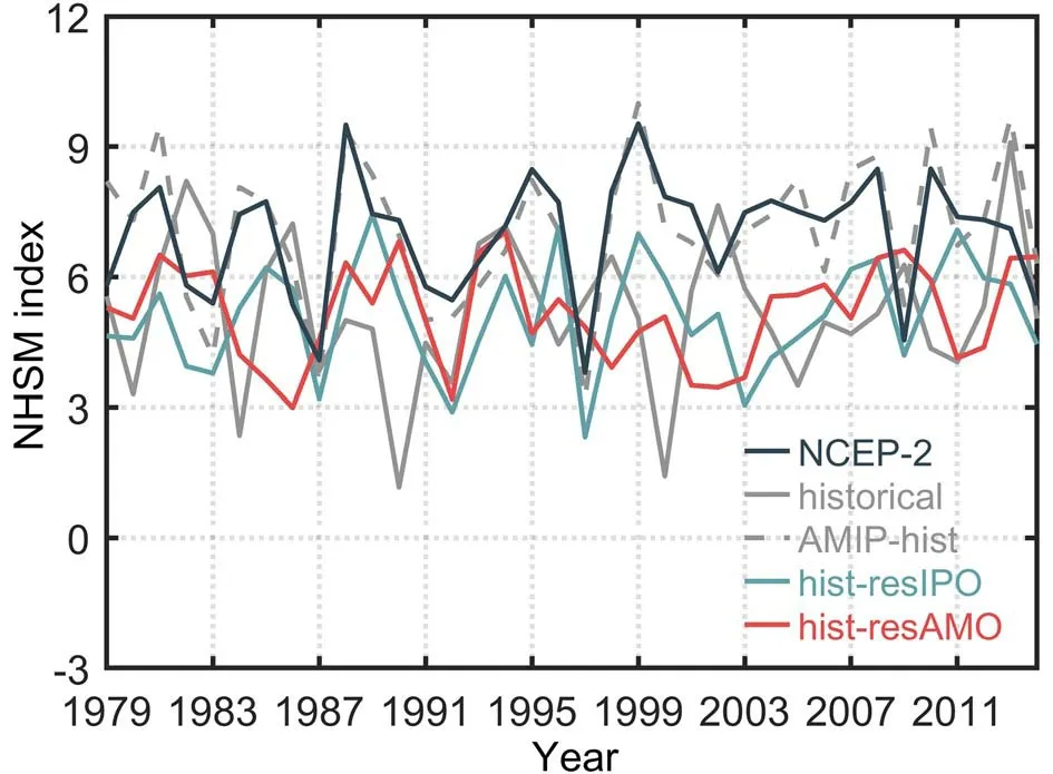
Fig. 5. Time series of boreal summer (March-June-July-August-September) mean NHSM circulation index measured by the vertical shear of zonal wind (850 hPa minus 200 hPa)averaged over (0°-20°N, 120°W-120°E) (Wang et al., 2013).The different lines represent the results from the NCEP-2 reanalysis dataset and each experiment.

Fig. 6. Differences in climatological (1979-2014) precipitation (shaded: units: mm d−1) and wind field at 850 hPa (vectors; units: m s−1): (a, b) between AMIP r1i1p1f1 and AMIP-TIP;(c, d) between AMIP r1i1p1f1 and AMIP-TIP-nosh; (e, f) between AMIP r1i1p1f1 and AMIP-hld r1i1p1f1. Panels (a), (c) and (e) show the summer (JJA) mean; (b), (d) and (f)show the winter (DJF) mean. The thick red line denotes the 500 m topographic height that is modified in AMIP-TIP, AMIP-TIP-nosh and AMIP-hld r1i1p1f1.

Fig. 7. Differences in climatological (1979-2014) precipitation (shaded: units: mm d−1) and wind field at 850 hPa (vectors; units: m s−1): (a, b) between AMIP r1i1p1f1 and AMIP-hld r1i1p1f2; (c, d) between AMIP r1i1p1f1 and AMIP-hld r1i1p1f3. Panels (a) and (c) show the summer (JJA) mean; (b) and (d) show the winter (DJF) mean. The thick red line denotes the 500 m topographic height that is modified in the AMIP-hld experiments.

Figure 7 shows the changes in rainfall and wind when removing the highlands over North and South America.According to the design of the GMMIP experiments, the effects of the Sierra Madre Mountains in North America and the Andes Mountains in South America on the formation of American monsoon are evaluated separately. The orographic forcing in North America generates a cyclonic circulation over the Sierra Madres with increased rainfall. Meanwhile, an anticyclonic circulation appears along the coast of Mexico with less rain (Fig. 7a). The change in precipitation in summer is more evident than in winter. In AMIP-hld r1i1p1f3, the Andes Mountains along the coast of South America higher than 500 m is set to 500 m. The difference in wind at 850 hPa shows a strong cyclonic anomaly over subtropical South America and a westerly wind anomaly over the eastern tropical Pacific. The decreased precipitation is situated over South America and the tropical Pacific from 10°N to 20°N, where the north ITCZ branch in summer is located(Fig. 7c). In DJF, there is more precipitation along the Andes Mountains and Panama strait, and less rainfall over the equatorial region. Previous studies suggest that the Andes is critical to the South American low-level jet and moisture transports over western South America (Junquas et al., 2016). Removing the Andes leads to a reduction in precipitation over the Andean Altiplano (Saurral et al., 2015). Our experiments present consistent results. As revealed in tier-3,the differences in low-level circulation and rainfall between AMIP r1i1p1f1 and AMIP-hld r1i1p1f3 show that more rainfall is distributed over this region when considering the orographic effect of the Andes.

3.4. Validation by Webster Yang index

Fig. 8. Climatological annual cycle of the WYI from 1979-2014. The black line is based on NCEP-2 reanalysis data, and the different colored lines represent the results in each experiment of GMMIP. The dashed color lines denote CGCM results, and solid color lines are based on AGCM outputs.

The Webster Yang index (WYI) is used to quantitatively describe the changes in monsoon circulation intensity between the perturbation experiments and control simulations. Calculated by the zonal wind shear between 850 and 200 hPa in the tropical Indian Ocean (0°-20°N,40°E-110°E), the WYI mainly indicates the variations in Asian summer monsoon (Webster and Yang, 1992). The climatological annual cycle of the WYI is shown in Fig. 8.The index increases from April, which indicates the onset of summer monsoon circulation, and reaches a peak in July.The WYI decreases from September to December with the summer monsoon retreat. It is found that FIO-ESM v2.0 can successfully reproduce the annual cycle of WYI, whether in CGCM or AGCM experiments. Comparing the historical and AMIP-hist results, the AGCM forced by observed SST and sea ice presents good ability in simulating WYI during summer monsoon onset periods. The WYI from March to June in the AMIP-hist run is consistent with NCEP-2 reanalysis data. However, the monsoon onset and peak in the historical run are delayed for about one month. For the CGCM,the model considering the air-sea interaction processes performs better than the AGCM in simulating the monsoon intensity in the peak and retreat seasons.

The thermal and mechanical forcings of the TIP topography play an important role in the Asian summer monsoon. In the AMIP-TIP and AMIP-TIP-nosh orographic perturbation experiments, WYI is significantly decreased during the summer monsoon season, which means the simulated intensity of monsoon is reduced compared with AMIP-hist results. In addition, the onset of summer monsoon is also delayed in those two experiments. Modifying topographies by leveling off the TIP to 500 m or removing surface sensible heating have the same effects on the simulation of WYI. The topography of the African highlands,Sierra Madre in North America, and the Andes in South America, have almost no effects on WYI simulation.

4. Usage notes

The tier-1 experiment of GMMIP aims to present the historical evolution of global monsoons since SST and sea ice are prescribed. It provides a platform to evaluate the capability of climate models in reproducing the monsoon mean state and the forced response to anthropogenic forcing when compared with tier-2 and historical experiments. Tier-2 shows the decadal variability (IPO and AMO) contributions to the monsoon system. How the decadal variability influences the global monsoon circulation and rainfall variation can be investigated. We suggest that the hist-resIPO and hist-resAMO simulations are compared with historical experiments of DECK. Furthermore, the topography has a great influence on global monsoons. The influences of dynamical and thermal forcing of the plateau or hilly terrain on the monsoon system and the hydrological cycle are still unclear.Tier-3 offers an opportunity to study the effects of topographic forcing, as well as the surface thermal status, on the monsoon system in different regions. We recommend that the AMIP-TIP, AMIP-hld, and AMIP-TIP-nosh outputs are compared with the AMIP r1i1p1f1 experiment, because the model settings and initial state in both experiments are consistent.

Comparison between AMIP-hist and tier-2 experiments provides a wealth of information about how the air-sea interactions influence the monsoon simulations on different time scales. In the aspect of monsoon mean state, the coupled runs considering air-sea interactions perform better in simulating the intensity of WYI in peak and retreat seasons compared with AMIP-hist results (Fig. 8). The simulations with real SST and sea ice are generally more skillful in simulating the interannual and interdecadal variation of the NHSM index (Fig. 5). This demonstrates that accurate boundary conditions and reasonable consideration of air-sea interaction are also very important for monsoon simulations on the interannual and interdecadal time scales.

The AGCM outputs with the original model grids (288 ×192) are provided by FIO-ESM v2.0. The output variables of tier-1 and tier-3 based on the AGCM are shown in Table 3.Tier-2 based on the CGCM not only includes the outputs from the atmospheric model, but also from the ocean, sea ice and ocean surface wave model. Detailed information is shown in Table 4. The dataset format is a generic data type,NetCDF-4, which is easily read by commonly used soft-ware. To check whether the orographic experiments are conducted correctly, we present all orographic modifications in the AMIP-TIP and AMIP-hld experiments. As shown in Fig. 6 and Fig. 7, the highlands in the region enclosed by the red lines is modified to 500 m in each orographic perturbation experiment.

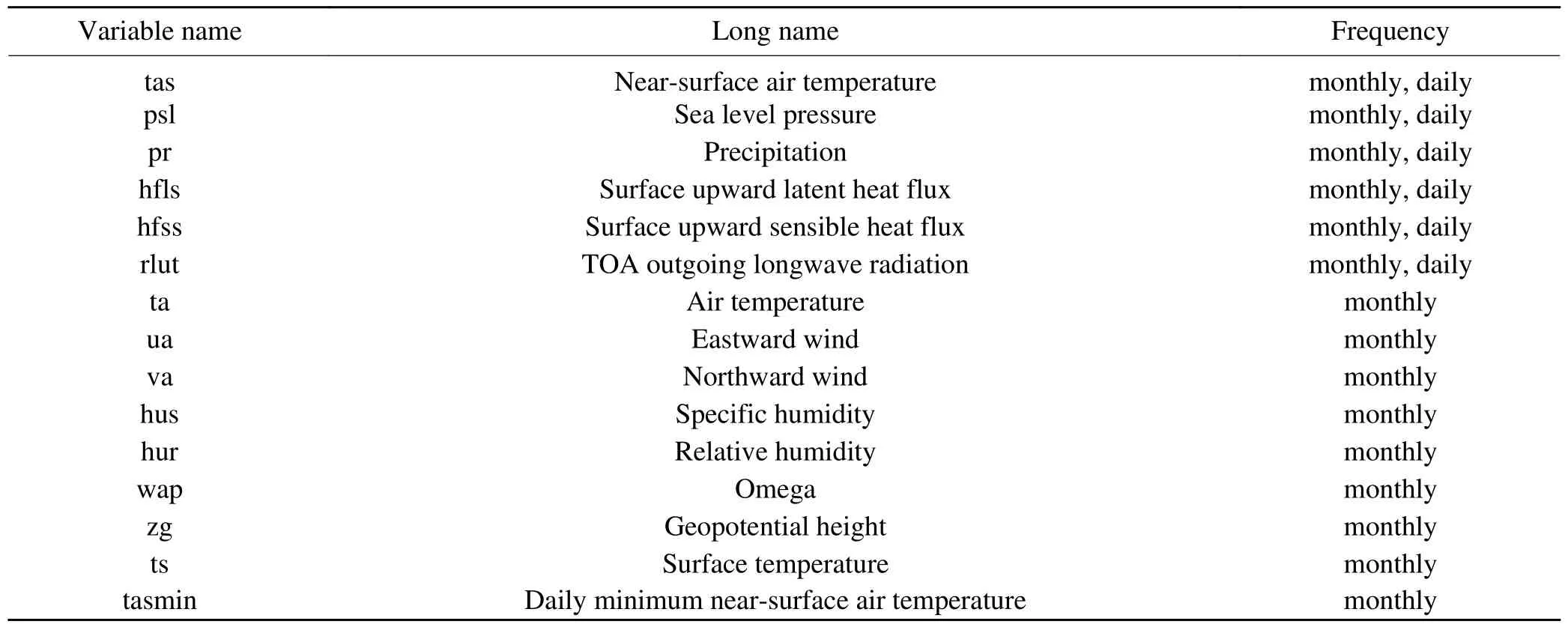
Table 3. FIO-ESM 2.0 outputs for tier-1 and tier-3 AGCM experiments.

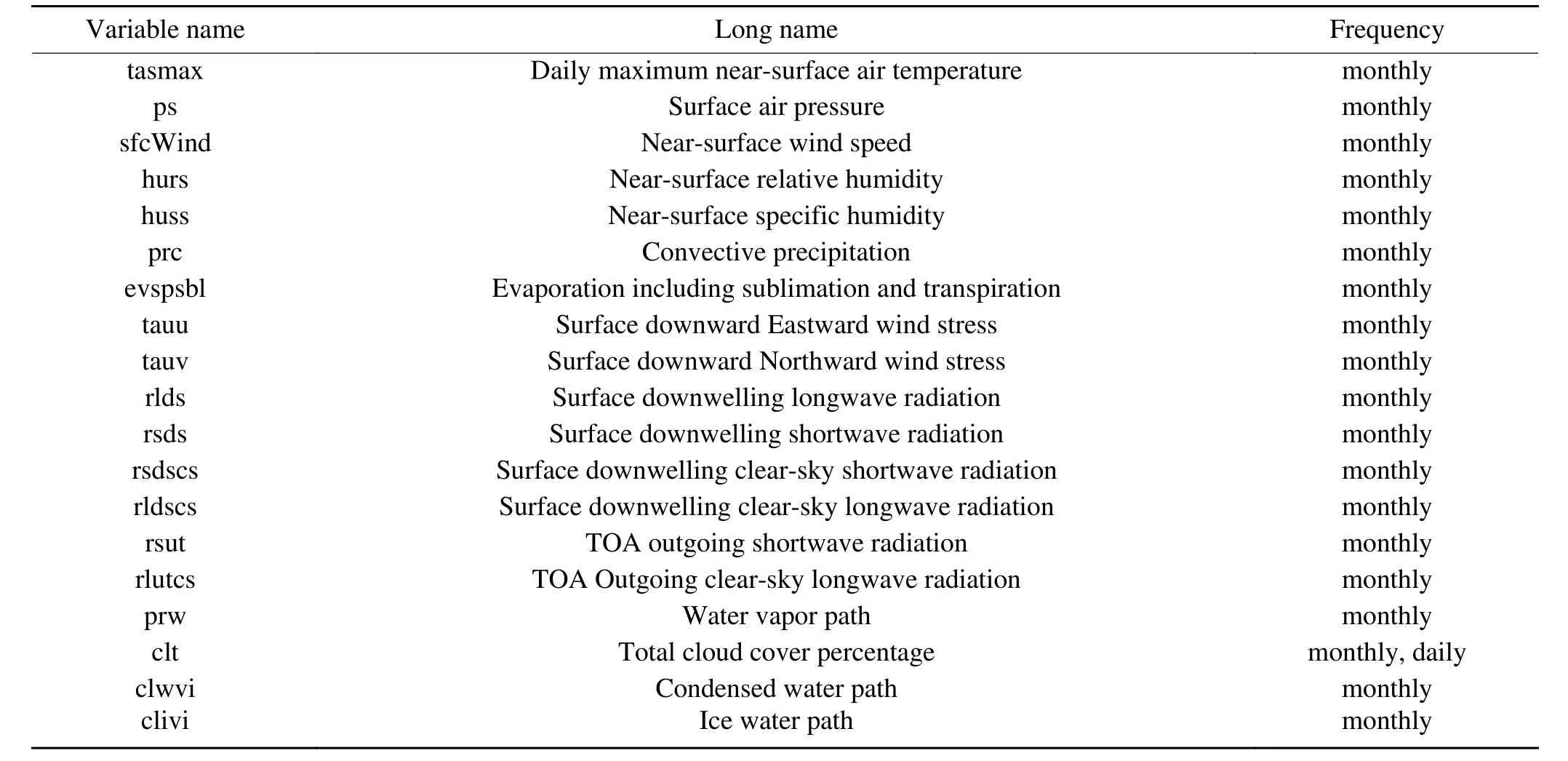
Table 3. (Continued.)

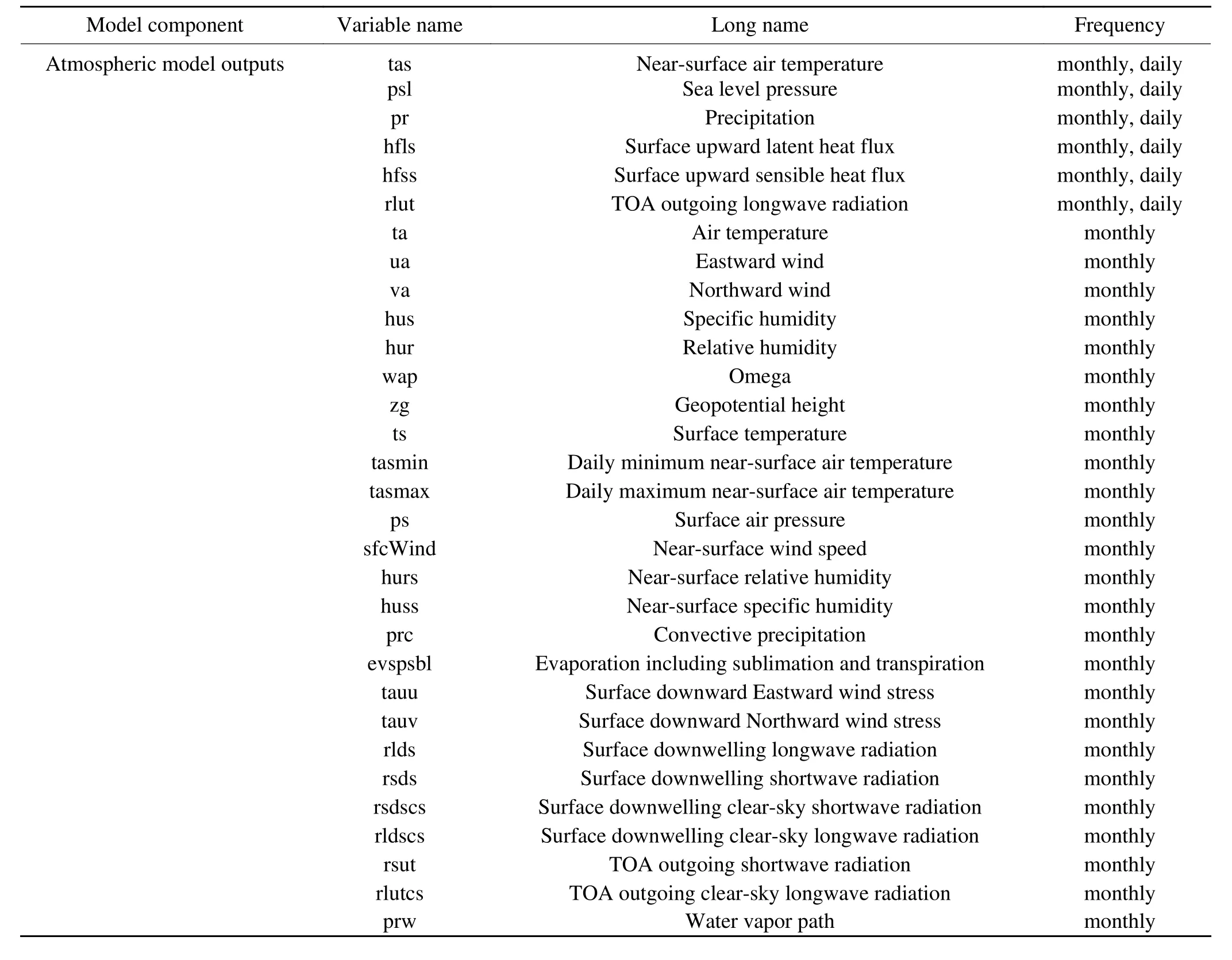
Table 4. FIO-ESM 2.0 outputs for tier-2 CGCM experiments.

Table 4. (Continued.)

Acknowledgements.This research was jointly supported by the National Key Research and Development Program of China(Grant No. 2017YFC1404004), the Project of Indo-Pacific Ocean Environment Variation and Air-sea Interactions (Grant No. GASIIPOVAI-06), the Basic Scientific Fund of the National Public Research Institute of China (Grant No. 2019S06). Ying BAO was supported by the National Key Research and Development Program of China (Grant No. 2016YFA0602200). Zhenya SONG was supported by the National Natural Science Foundation of China(Grant No. 41821004), the Basic Scientific Fund of the National Public Research Institute of China (Grant No. 2016S03), and the China-Korea Cooperation Project on Northwestern Pacific Climate Change and its Prediction. All numerical experiments were carried out at the Beijing Super Cloud Computing Center (BSCC).

Data availability statement

The data that support the findings of this study are available from https://esgf-node.llnl.gov/projects/cmip6/. All datasets are available to search and download via any one of the following portals:

USA, PCMDI/LLNL (California) -- https://esgf-node.llnl.gov/search/cmip6/

France, IPSL--https://esgf-node.ipsl.upmc.fr/search/cmip6-ipsl/

Germany, DKRZ--https://esgf-data.dkrz.de/search/cmip6-dkrz/

UK, CEDA--https://esgf-index1.ceda.ac.uk/search/cmip6-ceda/

Disclosure statement

No potential conflict of interest was reported by the authors.

Open Access This article is distributed under the terms of the Creative Commons Attribution 4.0 International License (http://creativecommons.org/licenses/by/4.0/), which permits unrestricted use, distribution, and reproduction in any medium, provided you give appropriate credit to the original author(s) and the source,provide a link to the Creative Commons license, and indicate if changes were made.