FGOALS-g3 Model Datasets for CMIP6 Flux-Anomaly-Forced Model Intercomparison Project

Yaqi WANG, Zipeng YU, Pengfei LIN, Hailong LIU*, Jiangbo JIN, Lijuan LI, Yanli TANG,Li DONG, Kangjun CHEN, Yiwen LI, Qian YANG, Mengrong DING, Yao MENG,Bowen ZHAO, Jilin WEI, Jinfeng MA, and Zhikuo SUN

1State Key Laboratory of Numerical Modeling for Atmospheric Sciences and Geophysical Fluid Dynamics,Institute of Atmospheric Physics, Chinese Academy of Sciences, Beijing 100029, China

2College of Earth and Planetary Sciences, University of Chinese Academy of Sciences, Beijing 100049, China

3International Center for Climate and Environment Sciences, Institute of Atmospheric Physics,Chinese Academy of Sciences, Beijing 100029, China

4School of Atmospheric Sciences, Guangdong Province Key Laboratory for Climate Change and Nature Disaster Studies,Sun Yat-sen University, Guangzhou 510275, China

ABSTRACT The Flux-Anomaly-Forced Model Intercomparison Project (FAFMIP) is an endorsed Model Intercomparison Project in phase 6 of the Coupled Model Intercomparison Project (CMIP6). The goal of FAFMIP is to investigate the spread in the atmosphere-ocean general circulation model projections of ocean climate change forced by increased CO2, including the uncertainties in the simulations of ocean heat uptake, global mean sea level rise due to ocean thermal expansion and dynamic sea level change due to ocean circulation and density changes. The FAFMIP experiments have already been conducted with the Flexible Global Ocean-Atmosphere-Land System Model, gridpoint version 3.0 (FGOALS-g3). The model datasets have been submitted to the Earth System Grid Federation (ESGF) node. Here, the details of the experiments,the output variables and some baseline results are presented. Compared with the preliminary results of other models, the evolutions of global mean variables can be reproduced well by FGOALS-g3. The simulations of spatial patterns are also consistent with those of other models in most regions except the North Atlantic and the Southern Ocean, indicating large uncertainties in the regional sea level projections of these two regions.

Key words: FAFMIP, CMIP6, global mean sea level rise, dynamic sea level change

1. Background and summary

Understanding changes in global and regional sea levels is of paramount importance, as they both reflect the natural and anthropogenic changes in the climate system and affect the livelihoods of people in coastal areas (Church et al., 2013). One of the main causes of global mean sea level rise (GMSLR) is ocean thermal expansion, with the rest mostly due to the loss of land ice. Based on phase 5 of the Coupled Model Intercomparison Project (CMIP5) multimodel mean, thermosteric sea level related to ocean thermal expansion accounts for 30%-50% of GMSLR during the 21st century (Church et al., 2013). In contrast, the redistribution of ocean salt content makes no significant contribution to GMSLR or its uncertainty (Gregory et al.,2016). On a regional basis, sea level change can deviate significantly from the global mean. Changes in dynamic sea level (DSL) induced by ocean circulation and density changes are the main contributors to the deviation. Sea level projections from CMIP5 have a considerable model spread at the regional scale, mostly caused by the differences in ocean density and redistribution by ocean circulation(Gregory et al., 2016).

To investigate the spread and isolate the uncertainty in sea level projections at both the global and regional scales,the Flux-Anomaly-Forced Model Intercomparison Project(FAFMIP) has been proposed by comparing results from atmosphere-ocean general circulation model (AOGCM)experiments with independent surface flux perturbations imposed on the sea surface (Gregory et al., 2016). FAFMIP is an endorsed Model Intercomparison Project of phase 6 of the Coupled Model Intercomparison Project (CMIP6). The Flexible Global Ocean-Atmosphere-Land System model,gridpoint version 3.0 (FGOALS-g3) (Li et al., 2020)developed at the State Key Laboratory of Numerical Modeling for Atmospheric Sciences and Geophysical Fluid Dynamics (LASG), Institute of Atmospheric Physics (IAP),Chinese Academy of Sciences (CAS), is one of the climate system models contributing to CMIP6. The FAFMIP experiments are also conducted using FGOALS-g3 following the standard protocol of Gregory et al. (2016), and the data have been submitted to the Earth System Grid Federation(ESGF) data server (https://esgf-node.llnl.gov/projects/cmip6/). The required diagnostics of FAFMIP are provided in the format of the CMIP6 Ocean Model Intercomparison Project (Griffies et al., 2016).

The purpose of this paper is to provide a comprehensive description of the FGOALS-g3 FAFMIP datasets for the users of CMIP6 datasets. The remainder of this paper is organized as follows. Section 2 presents the model descriptions and experimental design. Section 3 presents the basic technical validation of the FGOALS-g3 experiments. Section 4 describes the datasets. The fifth part provides usage notes.

2. Model and experiments

2.1. Introduction to the model

FGOALS-g3 has four component models: the Grid-Point Atmospheric Model of LASG-IAP, version 3(GAMIL3) for the atmosphere (Li et al., 2013), the LASG-IAP Climate System Ocean Model, version 3(LICOM3) for the ocean (Lin et al., 2016; Yu et al., 2018;Lin et al., 2020), the Los Alamos sea ice model, version 4(CICE4) for the sea ice, and the CAS Land Surface Model(CAS-LSM) for the land (Xie et al., 2018). All the components are coupled with version 7 of the flux coupler developed at the National Center for Atmospheric Research(Craig et al., 2005).

GAMIL3 uses a finite difference dynamical core,which conserves mass and effective energy under the standard stratification approximation. The horizontal resolution of GAMIL3 is ～2° (180×80) and the number of vertical layers used in GAMIL3 is 26. The land component is CASLSM with the same grid as GAMIL3. With regard to the physical processes of GAMIL3 and CAS-LSM, the details can be found in Li et al. (2020).

The ocean component, LICOM3, has also been extensively improved (Liu et al., 2012; Lin et al., 2016, 2020; Yu et al., 2018; Lin et al., 2020). Its dynamic core with a latitude-longitude grid structure is replaced by arbitrary orthogonal curvilinear coordinates (Yu et al., 2018). Therefore,the tripolar grid from Murray (1996) can be applied in LICOM3 with two North Poles on the Eurasian (65°N,65°E) and North American (65°N, 115°W) continents. The introduction of the tripolar grid can directly improve the effectiveness of the dynamic core by both enlarging the time steps and removing the zonal filter for momentum and tracers. An Arakawa B-grid is used for the horizontal grid with 360×218 grid points. The eta coordinates with 30 or 80 layers are used in the vertical direction, but only 30 layers are used for the DECK and FAFMIP experiments of CMIP6. With regard to the physical processes, the St.Laurent et al. (2002) internal tidal mixing is introduced into LICOM3 (Yu et al., 2017), and the buoyancy frequencyrelated thickness diffusivity of Ferreira et al. (2005) is applied in the eddy-induced advection of Gent and McWilliams (1990). In addition, the chlorophyll-a-dependent solar penetration of the Ohlmann (2003) scheme and vertical mixing of Canuto et al. (2002) are inherited from LICOM2.CICE4 is the sea ice component of FGOALS-g3, with the same horizontal resolution as the ocean component.

2.2. Experimental design

Five experiments are carried out in FAFMIP: faf-water,faf-stress, faf-heat, faf-all and faf-passiveheat (Table 1). In the first three experiments, the surface momentum, freshwater and heat flux perturbations are applied, while in faf-all,all three perturbations are applied together. All the forcing data are from Gregory et al. (2016), which are monthly flux anomalies of the ensemble mean of the 61st-80th years 1pctCO2 experiments from 13 CMIP5 models. For comparison between the perturbation and preindustrial control(piControl) experiments, all other conditions of the experiments are the same as those of the setup of the piControl run, including the point to branch the experiment, the concentration of CO2(280 ppm), etc. The experiments are all 70 years long, and the scale of the CO2concentration is doubling. The control experiment used in this paper is the faf-passiveheat experiment, which is equivalent to the piControl run but with an extra diagnostic tracer. The details of the five FAFMIP experiments are described as follows:

Table 1. Descriptions of the FAFMIP experiments.

In the faf-stress experiment, the perturbations of surface downward fluxes of eastward and northward momentum derived from CMIP5 are applied in the surface zonal and meridional momentum flux. The stress perturbations are directly added to the momentum balance of the seawater but not to the ocean subgrid processes and the momentum balance of the sea ice. Figure 1a shows the annual mean surface momentum flux perturbations for FAFMIP. Its dominant feature is the increase in westerly wind stress in the Southern Ocean, which indicates that large changes in faf-stress will occur in the Southern Ocean.

In the faf-water experiment, a perturbation of freshwater anomalies is applied to the freshwater flux into the sea surface. The anomalies are the sum of all possible sources in the CMIP5 AOGCM, including precipitation, evaporation,river inflow and water fluxes between floating ice (sea ice and icebergs) and seawater. Figure 1b shows the annual mean surface water flux perturbations for FAFMIP. We find that its pattern is dominated by that of precipitation changes, which are positive near the equator and at mid to high latitudes and negative in the subtropics.

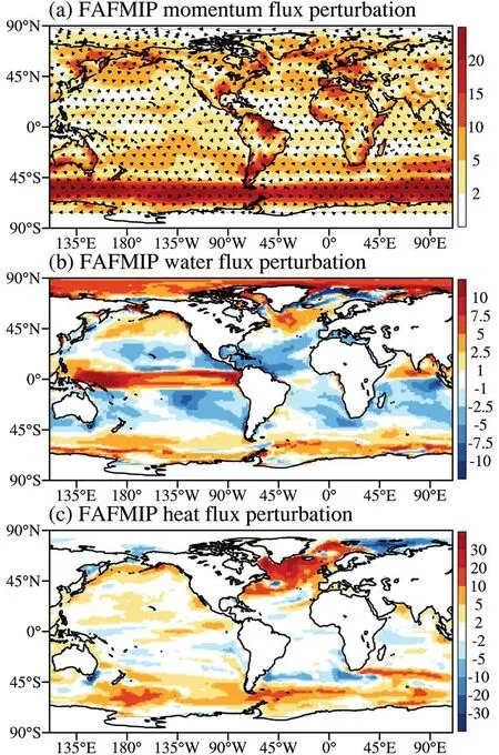
Fig. 1. Surface flux perturbations of (a) momentum (10−3 Pa,color indicates the magnitude of the vector, arrow indicates direction), (b) water (10−6 kg m−2 s−1) and (c) heat (W m−2)from FAFMIP.

In the faf-heat experiment, a perturbation of the surface downward heat flux in seawater is applied to the heat flux into the sea surface. The anomalies are the sum of all possible sources in the CMIP5 AOGCM, including the net downward radiative fluxes, sensible and latent heat fluxes to the atmosphere, and heat fluxes between sea ice and seawater.In previous studies, we found that there is a negative feedback due to the air-sea interaction at the surface, which will reduce the increase in temperature by approximately 50%.To avoid this effect, a passive tracer, which cannot feel heat perturbation, has been introduced to compute the surface heat flux instead of the sea surface temperature (SST), as proposed by Bouttes et al. (2014). The passive tracer is initialized to the ocean temperature at the start of the experiment and subsequently transported by all the same processes as ocean temperature, except for the heat anomalies. Figure 1c shows the annual mean surface heat flux perturbations for FAFMIP. Large positive anomalies occur in the North Atlantic Ocean and the Southern Ocean.

In the faf-all experiment, the surface flux perturbations of momentum, heat and freshwater are all applied simultaneously into the seawater. The method of computing surface flux uses the same method as that in the faf-heat experiment. The purpose of the faf-all experiment is to quantify the nonlinearities of the effects of the three perturbations. If the ocean response to CO2forcing may be interpreted as the sum of the effects, the effects of the three perturbations are linear.

In faf-passiveheat, the heat flux perturbation is applied instead to a passive tracer to diagnose the effect of added heat on the ocean temperature through processes other than heat transport due to circulation. The tracer here is initialized to zero and does not affect the processes. Therefore,the faf-passiveheat experiment is the same as the standard piControl but with an additional passive tracer for diagnosis. The results of this experiment are used as a reference in the present paper.

Three additional experiments, faf-heat-NA50pct, fafheat-NA0pct and faf-antwater-stress for FAFMIP, which were further proposed by the FAFMIP meeting in April 2019, have not been conducted so far. Therefore, they are not included and discussed in the present paper. The former two experiments reduce the double-counted surface heat flux in the North Atlantic due to the change in SST. The latter experiment is to investigate the effects of both wind stress and freshwater in the Southern Ocean. Further details of the implementation of each of the experiments can be found at the following website: http://www.fafmip.org.

3. Validation

Some preliminary results from the experiments are validated here, and the usefulness of this dataset is demonstrated.The metrics shown here follow Gregory et al. (2016), including the global mean of SST changes, ocean heat content(OHC) change, DSL change and the maximum transport change of Atlantic meridional overturning circulation(AMOC), as well as the spatial pattern of zonal mean temper-ature change, OHC change and DSL change. All the changes are relative to the piControl (or faf-passiveheat)state, the values of the 70-year mean or values of the corresponding year are used for the time series of changes, and the values of the 61-70-year mean are used for the spatial patterns of changes.

3.1. Time series of changes

3.1.1.Global mean SST

The global mean SST change with respect to piControl reaches approximately 0.9 K after the 70th year in the fafall experiments (Fig. 2a, black line). The change in faf-all is mainly dominated by faf-heat but with a slightly smaller magnitude (approximately 0.8 K after the 70th year, Fig. 2a, red line), while the changes in global mean SST are almost negligible in both faf-stress (Fig. 2a, orange line) and faf-water(Fig. 2a, blue line). Under faf-stress, the changes in global mean SST slow down gradually and decrease by 0.07 K after the 70th year. In faf-water, the global mean SST levels off within approximately 30 years, showing a decrease of almost the same magnitude as that of faf-stress (−0.06 K)after the 70th year.

3.1.2.Global OHC

The OHC is defined as the vertical integration of ocean temperature from the sea surface to the bottom, multiplied by the reference density (1026 kg m−3) and the specific heat capacity (3992 J kg−1°C−1). Changes in globally integrated OHC are crucial for the GMSLR induced by thermal expansion. The time series of globally integrated OHC change in faf-all (Fig. 2b, black line) is still dominated by faf-heat(Fig. 2b, red line), reaching approximately 0.9 YJ (1 YJ =1024J) after the 70th year for both experiments. Changes in globally integrated OHC are also negligible in faf-stress(Fig. 2b, orange line) and faf-water (Fig. 2b, blue line), in which they both increase only approximately 0.1 YJ at the end of the experiments.

The globally integrated OHC change is proportional to the global mean ocean temperature change, which is also shown in Gregory et al. (2016, second row of their Fig. 5).Their values have a range of 0.2-0.3 K in faf-heat for five CMIP5 models in the last year of integration, while the value in our experiment is relatively small at approximately 0.16 K. This might be due to the larger negative changes in the sea ice cover or SST of FGOALS-g3 than that of other models.

3.1.3.DSL

In the present study, DSL (ζ) is defined as the deviation of the sea surface height (η) from the global mean (η¯);that is, ζ=η−η¯. To quantify the DSL change in FAFMIP experiments, we compute the time series of the areaweighted spatial standard deviation of the annual mean DSL change of each experiment (Fig. 2c). The large values mean that the spatial pattern of forced change in DSL can be detected from the background of unforced variability. The DSL rises above the control value in all four experiments. It is also the case for the above two variables that the large DSL changes in faf-heat (Fig. 2c, red line) can explain most of the changes in faf-all (Fig. 2c, black line), with values of 0.10 m and 0.11 m, respectively. The magnitudes of the DSL change of faf-all in this study are near the upper limit of the values in Gregory et al. (2016). The faf-stress and fafwater values do not differ significantly from those of the control, with values less than half of those of the other two runs, faf-stress and faf-water.

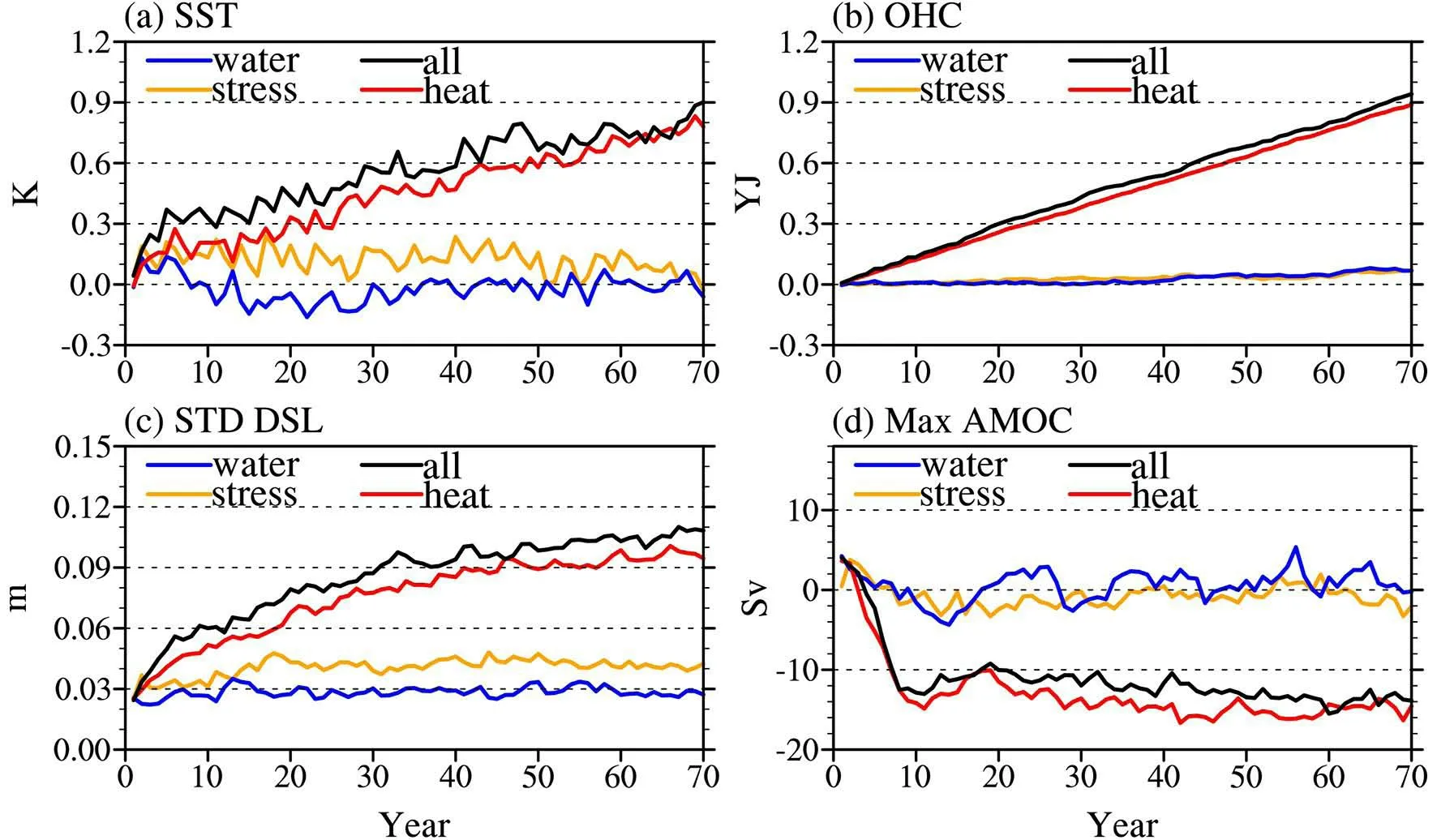
Fig. 2. Global annual time series for faf-stress (orange), faf-water (blue), faf-heat (red) and faf-all (black)experiments: (a) SST change (K); (b) ocean heat content change (YJ); (c) the spatial standard deviation of dynamic sea level change; and (d) maximum of the Atlantic meridional overturning streamfunction (Sv). The changes in (a-d)are with respect to the 70-year mean of piControl (or faf-passiveheat), while (b) is with respect to the corresponding year of the piControl run.

3.1.4.AMOC

The evaluations of the maximum transport of AMOC change for FAFMIP experiments are shown in Fig. 2d,which is crucial to determine the changes in OHC and sea level in the North Atlantic. The weakened AMOC can be seen in both faf-heat (Fig. 2d, red line) and faf-all (Fig. 2d,black line), in which the maximum AMOC weakens nearly 14 Sv at the end of the experiments. The change in faf-heat is also within the range of 5-15 Sv in Gregory et al. (2016,third row of their Fig. 5). In faf-stress (Fig. 2d, orange line)and faf-water (Fig. 2d, blue line), the changes in the maximum AMOC relative to the control are less than 1 Sv at the 70th year, indicating that the perturbations to the surface momentum and water fluxes do not cause significant changes in the AMOC.

The weakened AMOC in faf-heat is larger than the expected response for the 1pctCO2 experiments. This is due to the positive feedback between the surface heat flux and the weakening of the AMOC. When the AMOC declines, the associated heat transport decreases, and the SST cools in the North Atlantic. The cooling SST inhibits the heat flux from being released into the atmosphere, and the ocean absorbs more heat flux, which will further decrease the AMOC.Another reason for a larger response than that in 1pctCO2 is that the heat flux perturbation consistent with double CO2concentration is applied at the beginning of the faf-heat experiment, while the CO2concentration in 1pctCO2 is gradually increased to double.

3.2. Spatial patterns of changes

3.2.1.Zonal mean ocean temperature

Figure 3 shows the change in zonal mean ocean temperature in the time mean of the 61st-70th year relative to the piControl run. The warming occurs in faf-all in the upper 1000 m at most latitudes (Fig. 3d), with the maximum magnitude of changes over 1 K at the surface at approximately 60°N. The warming of faf-all is mainly dominated by fafheat (Fig. 3c), and faf-water contributes 0.2 K between 10°and 60°N at depths of approximately 200-600 m (Fig. 3b).It is unusual that the significant warming induced by the surface heat perturbation penetrates 4000 m in the Arctic Ocean, which cannot be found in the results of Gregory et al. (2016). We presume that this might be due to the large vertical mixing in this region, and it is worth investigating further.

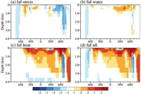
Fig. 3. Changes in zonal mean ocean temperature (K) as a function of depth and latitudes of the time mean during the last 10 years (61-70) of (a) faf-stress, (b) faf-water, (c) faf-heat and (d) faf-all relative to the piControl run.

The cooling occurs in faf-all in three regions: south of 60°S from the surface to 4000 m, approximately 70°N in the subsurface from 1000 m to 3500 m, and at the bottom(Fig. 3d). Three kinds of perturbations at the surface all possibly contribute to the negative changes. The cooling south of 60°S is attributed to both faf-stress and faf-water, while the cooling in the high latitudes of the Northern Hemisphere is dominated by both faf-stress and faf-heat. The small negative temperature changes at the bottom are due to faf-heat. The cooling in the high latitudes might be related to the weakened circulation. Most of the cooling patterns are also consistent with the multimodel mean results from Gregory et al. (2016), while cooling below 1000 m in the Northern Hemisphere high latitudes in faf-heat does not appear in FGOALS-g3, and cooling south of 60°S in fafwater does not appear in the multimodel mean.

3.2.2.DSL and OHC

Change patterns of the DSL and OHC in the time mean of the 61st-70th year of the FAFMIP experiments relative to the piControl run are shown in Fig. 4 and Fig. 5, respectively. The heat flux perturbation produces the most changes in the spatial pattern of the DSL (Figs. 4c and d), while the wind stress and freshwater perturbations dominate the positive anomaly in the Southern Ocean and in the Arctic, respectively. Previous studies point out that the simulated common DSL features are the dipole in the North Atlantic, the enhanced sea level rise in the Arctic and the increase in the gradient across the Antarctic Circumpolar Current (ACC)(Church et al., 2013; Bouttes and Gregory, 2014). The pattern of DSL changes and the contribution of three flux perturbations are also the same as the results from Gregory et al. (2016).

There is a strong correlation between the patterns of OHC and DSL change in both faf-heat (Fig. 4c and Fig. 5c)and faf-all (Fig. 4d and Fig. 5d). This is consistent with previous studies, suggesting that the patterns of OHC change and corresponding DSL change are largely driven by surface heat flux perturbations (Gregory et al., 2016). As discussed in section 3.1.4, there is also a similarity of the AMOC response between faf-heat and faf-all. The regional OHC changes are relatively small in faf-stress (Fig. 5a) and fafwater (Fig. 5b) in comparison to those of faf-heat (Fig. 5c)and faf-all (Fig. 5d).

The differences between FGOALS-g3 and the multimodel mean of Gregory et al. (2016) appear in the fafwater experiment. First, the water flux perturbation makes an opposite contribution to the dipole in the multimodel mean of Gregory et al. (2016), while it makes no significant contribution in FGOALS-g3. Second, the increase in the gradient across the ACC in the Southern Ocean is mainly caused by momentum flux perturbation and somewhat by the water flux perturbation in FGOALS-g3. The results of Gregory et al. (2016) show that freshwater perturbations reduce the gradient in the Southern Ocean. Combining these differences with the deviation in the zonal mean ocean temperature from the multimodel mean results discussed in section 3.2.1, we can find that the North Atlantic and the Southern Ocean are the two regions with large uncertainties in sea level projections.

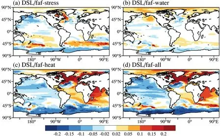
Fig. 4. Changes in dynamic sea level (m) averaged duing the last 10 years (61-70) of (a) faf-stress, (b) faf-water, (c)faf-heat and (d) faf-all relative to the piControl run.

Fig. 5. Changes in ocean heat content (GJ m−2) averaged duing the last 10years (61-70) of (a) faf-stress, (b) fafwater, (c) faf-heat and (d) faf-all relative to the piControl run.

4. Data records

FAFMIP datasets have been uploaded onto the ESGF node and can be found at https://esgf-node.llnl.gov/projects/cmip6/. The dataset format is Network Common Data Form(NetCDF), version 4. Although the model outputs have double precision, we converted all the variables into single precision for analysis. These data can be easily dealt with by common computer programming languages and professional software such as Climate Data Operators (CDO,https://code.mpimet.mpg.de/projects/cdo/) or NetCDF Operator (NCO, http://nco.sourceforge.net).

5. Usage notes

The original model outputs are on a tripolar grid with two poles in the Northern Hemisphere on the continents.The horizontal grid numbers are 360 and 218 in the zonal and meridional directions, respectively. The original grid distribution is kept and the format is slightly changed to Climate Model Output Rewriter (CMOR) file structure as required by FAFMIP. The data have 30 vertical levels, and the original vertical level is not changed on the ESGF note.The first level is at a depth of 5 m with a thickness of 10 m.The variables of Priority 1 for FAFMIP are shown in Table 2.

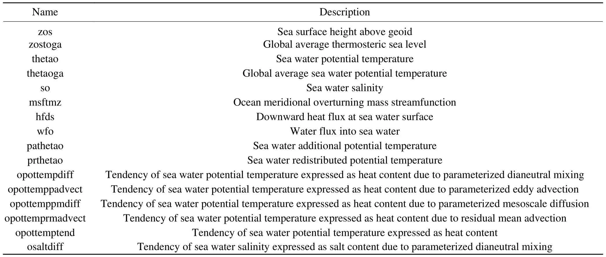
Table 2. Descriptions of output variables of Priority 1 for FAFMIP.

Table 2. (Continued.)

Acknowledgments.This study was supported by National Key R&D Program for Developing Basic Sciences(2018YFA0605703), the Strategic Priority Research Program of Chinese Academy of Sciences (Grant No. XDB42010404) and the National Natural Science Foundation of China (Grants 41976026,41776030 and 41931183, 41931182). The authors acknowledge the technical support from the National Key Scientific and Technological Infrastructure project "Earth System Science Numerical Simulator Facility" (EarthLab).

Data availability statement

The data that support the findings of this study are available from https://esgf-node.llnl.gov/projects/cmip6/.

The citation faf-stress is “CAS FGOALS-g3 model output prepared for CMIP6 FAFMIP faf-water. Earth System Grid Federation. http://doi.org/10.22033/ESGF/CMIP6.3299”.

The citation faf-water is “CAS FGOALS-g3 model output prepared for CMIP6 FAFMIP faf-stress. Earth System Grid Federation. http://doi.org/10.22033/ESGF/CMIP6.3297”.

The citation faf-heat is “CAS FGOALS-g3 model output prepared for CMIP6 FAFMIP faf-heat. Earth System Grid Federation. http://doi.org/10.22033/ESGF/CMIP6.3293”.

The citation faf-all is “CAS FGOALS-g3 model output prepared for CMIP6 FAFMIP faf-all. Earth System Grid Federation. http://doi.org/10.22033/ESGF/CMIP6.3291”.

The citation faf-passiveheat is “CAS FGOALS-g3 model output prepared for CMIP6 FAFMIP faf-passiveheat.Earth System Grid Federation. http://doi.org/10.22033/ESGF/CMIP6.3295”.

Disclosure statement

No potential conflict of interest is reported by the authors.

Open AccessThis article is distributed under the terms of the Creative Commons Attribution 4.0 International License (http://creativecommons.org/licenses/by/4.0/), which permits unrestricted use,distribution, and reproduction in any medium, provided you give appropriate credit to the original author(s) and the source, provide a link to the Creative Commons license, and indicate if changes were made.