Study on Rice Yield Estimation Model Based on Quantile Regression

Su Zhong-bin, Yan Yu-guang, Jia Yin-jiang, Sun Hong-min, Dong Shou-tian, and Cao Yu-ying

College of Electrical and Information, Northeast Agricultural University, Harbin 150030, China

Abstract: An airborne multi-spectral camera was used in this study to estimate rice yields. The experimental data were achieved by obtaining a multi-spectral image of the rice canopy in an experimental field throughout the jointing stage (July, 2017) and extracting five vegetation indices. Vegetation indices and rice growth parameter data were compared and analyzed. Effective predictors were screened by using signi ficance analysis and quantile and ordinary least square (OLS) regression models estimating rice yields were constructed. The results showed that a quantile regression model based on normalized difference vegetation indices (NDVI) and rice yields performed was best for τ=0.7 quantile. Thus, NDVI was determined as an effective variable for the rice yield estimation during the jointing stage. The accuracy of the quantile regression estimation model was then assessed using RMES and MAPE test indicators.The yields by this approach had better results than those of an OLS regression estimation model and showed that quantile regression had practical applications and research signi ficance in rice yields estimation.

Key words: quantile regression, multispectral image, rice yield, vegetation index

Introduction

Rice is a key food crop throughout China, it is therefore of considerable practical significance to be able to estimate rice yields scientifically and accurately in order to support agricultural and economic development. Improvements are necessary to both estimation accuracy and the cost of rice production. It is therefore important to enhance the estimation methods to assess rice yields (Li, 2018).Remote sensing (RS) spectroscopy applications develop rapidly in recent years and are now widely applied for crop yield estimations. Indeed, a range of studies from around the world have shown a strong correlation between crop yields and RS spectral data(Zhaoet al., 2012; Liuet al., 2017). In earlier work,Tanget al. (2015) extracted data on rice area using RS spectral data and estimated yield per unit area across an administrative region and the results showed an average yield estimation accuracy for Jiangsu Province of China that was as high as 99.46%. Thus,the comprehensive utilization of digital and spectral image processing technology enables the rapid and non-destructive collection of growth parameter data for crops including chlorophyll and nitrogen(Hanet al., 2012). In comparison with traditional RS technology, high resolution recent land spectral images have the advantages of low instrument costs as well as high image quality and convenience (Guoet al., 2011; Zhanget al., 2011; Li and He, 2009).Utilizing digital rice canopy images, Liet al.(2017)performed cluster analysis amongst some techniques to develop ak-means clustering algorithm and successfully extracted estimated values for the rice spike to develop a yield prediction model.

The ordinary least square (OLS) method is frequently used in traditional crop yield estimation approaches (Huanget al., 2011). The regression in this case; however, assumes that independent variables can only affect the position of the conditional distribution of dependent variables, but not any other aspects of the scale shape of their distributions (Chen and Ding, 2008). The linear hypothesis required by OLS method is quite extreme, so it will therefore not be fully met by many practical problems. This means it is hard to obtain unbiased and effective parameter estimates (Luo, 2009; Wanget al., 2017). Thus, in order to remedy the problems seen in OLS method,when performing a regression analysis, workers such as Koenker and Bassett (1978) proposed the use of the quantile regression method. Results in this case are more robust (i.e., independent of dependent variable outliers) and enable the permissiveness of preconditions to be applied (i.e., without making any assumptions about the distribution of random perturbations). Due to the richness of information afforded by this approach(i.e., the regression fitting results of dependent variables in any quantile given), this method is widely applied especially for the dependent variables with heteroscedasticity, rear tail and spike distributions (Qiao and Li, 2012). Quantile regression has been widely applied across many fields, but it has seldom been used to date for rice yield estimation. An unmanned aerial vehicle (UAV) platform near-ground spectral image was used in this analysis to obtain multiple vegetation indices. Univariate rice yield estimation models were then established by comparing these indices with ground data. A quantile regression rice yield estimation model suitable for different yield levels was developed by comparing the precision of OLS regression model.

Materials and Methods

Experimental field

The experiment was carried out in Donghe Jiuhong Science and Technology Demonstration Park in Qingan City, Heilongjiang Province, China. The rice variety selected for this study was Wuyou Dao4(Daohuaxiang 2) and this variety had a growth period of around 147 days (turning green tillers on June 25th,2017; jointing and booting on July 15th, 2017; heading and fl owering on August 10th, 2017; filling and fruiting on September 10th, 2017 and ripening to harvest on September 25th, 2017).

Testing scheme

The total length of the experimental field where the rice was grown was 210 m; six gradient fertilization treatments were used, N0, N1, N2, N3, N4 and N5.Compound fertilizer was used as the base for this experiment, while urea was applied at the tillering fertilizer. Conforming with local planting standards,35 kg compound fertilizer and 15 kg tillering fertilizer per hectare were utilized; the amounts applied are summarized in Table 1. Uniform fertilization was carried out in the test plot; all the experiments were performed in the same way and utilized a uni fied cultivation mode. Apart from fertilizer, all the management models were consistent with an ordinary field. No serious diseases, insect pests, drought, waterlogging or other extreme disasters were seen over the experimental period.

Data acquisition and processing

Data acquisition

An ADC-SNAP multispectral imaging system was used to obtain multispectral images from a six-rotor UAV. This UAV was flown at an altitude of 100 m over several sorties between 12: 00 p.m. and 2: 00 p.m.on the test day to ensure coverage of all the plots.Ground tests were then carried out synchronously on the day of aerial photography. Thus, the chlorophyll SPAD value and leaf nitrogen content (LNC) were measured using a SPAD-502 chlorophyll instrument.Five sample cells were taken from each test plot,from which five samples were taken in each case. The average value was recorded in each case, which was the average of SPAD and LNC values from each test plot. Rice plant height data were collected manually using the five-point cross sampling method. Plants were harvested at the end of September 2017 and the yields of rice harvested from each plot were measured.

Data processing

A total of 41 spectral images taken during the jointing stage were selected to screen and splice multispectral images; an entire image of the experimental field is shown in Fig. 1A. In the first place, multispectral images were corrected using gray-cloth reflectivity and processed final versions were calculated using the software ENVI, according to the formula presented in Table 2 (Zhang, 2017). Multispectral images corresponding to each vegetation index were obtained(Fig. 1B-F). According the region of interest (ROI)tool in this software, the rice canopy vegetation indices in each test plot were efficiently calculated.

Table 1 Fertilization amounts

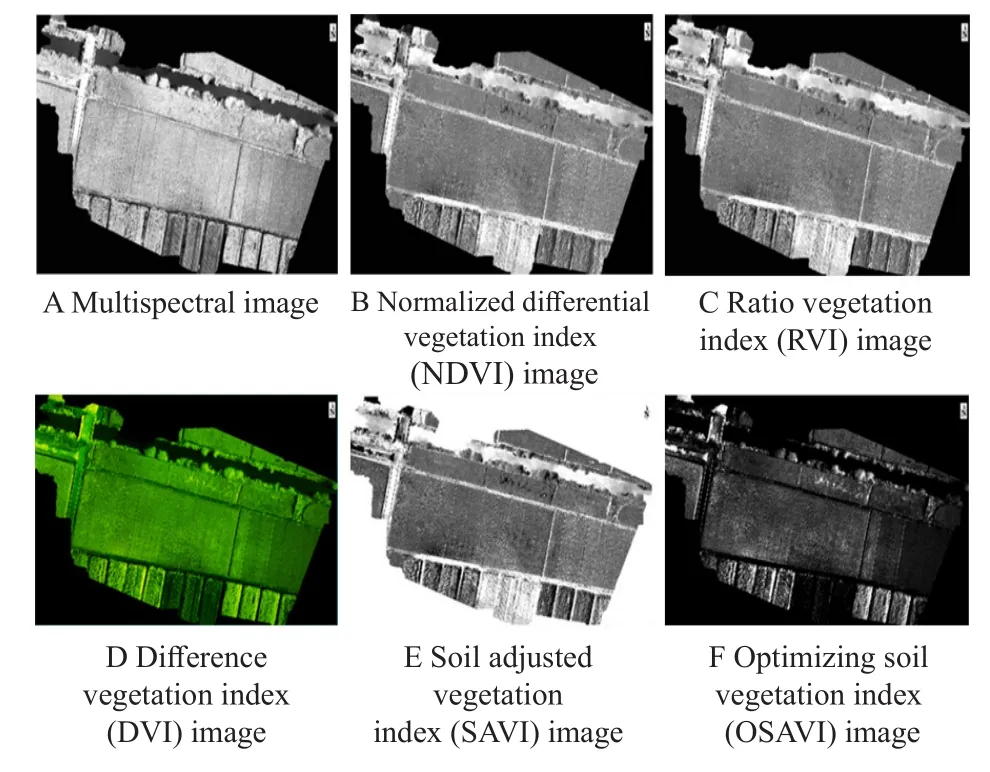
Fig. 1 Vegetation index images

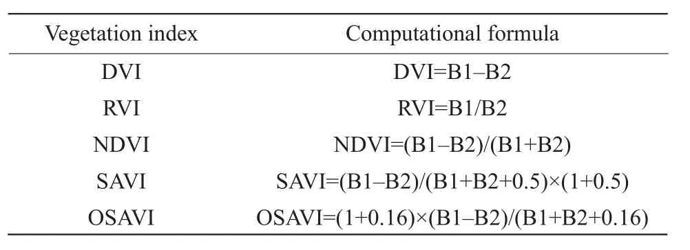
Table 2 Amounts of gradient fertilizer

Establishing an Estimation Model for Unit Yield

Quantile regression theory

The general basis of a quantile regression was first to obtain all the conditional quantiles of the dependent variable and then to use them at different distributional locations as standard to conduct the regression of an independent variable. A regression model under all the quantiles was therefore obtained for a group of random samples of the dependent variableY: {y1,y2,y3, …,yn}.

The regression criterion for sample mean regression to minimize the sum of squared errors was as the following:

The regression criterion for sample quantile regression to minimize the sum of absolute weighted errors was as the following:

The sample meanζwas used in this formula.

The starting point for regression was the basic definition of sample quantiles. Thus, by avoiding reliance on ordered sample observation sets, it was easy to extend this approach to linear models. Thus,given a set would contain a correlation between dependent and independent variablesX,Yin order to determine different values of the variableX, the random variableYhad a corresponding distribution functionF(Y|X).

Assuming that the random variableYwas comprised of continuous data and distribution function wasFy(y),thenτquantile was de fined as the following:

While, 0≤τ≤1, it was also suited. Thus, if all the quantile distributions were obtained in advance,the specific distribution of the dependent variableYcould be determined, according to the corresponding relationship between the quantile and its distribution function. This was the basis of the quantile regression method proposed by Koenker and Bassett (1978).

The speci fic analysis performed here was outlined;assuming thatτconditional quantile of the dependent variableYwas as the following:

Thus, whenFY|X(y) represented the conditional distribution of continuous dependent variableYunder specific independent variableX, thenQτ(Y|X) was a function ofX, denotedg(X)=Qτ(Y|X). This was applied by Koenker and Bassett (1978) who utilizedg(X) as a linear function ofX, as the followings:

The unknown parametersβ0(τ) satis fied the quantile constraintQτ(ε|X)=0. This model was therefore linear quantile regression.

The parameterβ0(τ) satisfied relationship as equation (7):

In this expression,ρτ(z)=z[τ-I(z＜0)] was referred to the check function, whileI(*) was the indicator function. This meant whenZwas true,Zwas false andρτ(z) was an asymmetric piecewise function (Fig. 2).The parameter estimate could be solved using equation(7). On this basis, given a value ofτ, a set of estimated values ofβ0(τ) could be obtained.

Quantile regression model

Four rice growth parameters (chlorophyll SPAD value, leaf nitrogen content LNC, plant height and leaf temperature) as well as five common vegetation indices (NDVI, RVI, DVI, SAVI and OSAVI) were selected as independent model variables while unit yield (kg · m-2) of each plot in the experimental field was used as the dependent variable (Y). The linear quantile regression model for each prediction variable and rice yield per unit area was initially established.This model then fitted regressions at different quantiles with step lengths of 0.1 (i.e., 0.1, 0.2, 0.3, 0.4, 0.5, 0.6,0.7, 0.8 and 0.9). Estimated values for constant and coefficient terms were calculated using the smoothing method in the parameter estimation algorithm(Fig. 3).

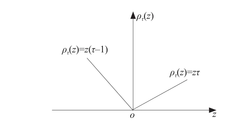
Fig. 2 Quantile regression loss function

The presentation in Fig. 3 showed that the estimated values of constant and coefficient terms for all the models under different quantiles fell within the confidence interval range and fluctuated around estimated values of corresponding OLS regression,which suggested that linear correlation between predicted variables and rice yield per unit area was different, when the yield was low, normal or high.

In the extremely low quantile range (τ＞0.2), the con fidence level of the whole partial digit regression model also remained low. However, as quantile increased, the confidence interval of the model contracted overall even though a slight rebound trend was seen within the extremely high quantile range(τ＞0.9). This analysis showed that predictors could be used to characterize different distributions of the dependent variable per unit yield. Quantile regression results revealed more robust performances in the case of outliers at both ends of the rice per unit yield distribution. Indeed, within quantile range (0.2＜τ＜0.8), this model could be roughly divided into three categories, according to the changes in confidence interval. In category one, the model confidence interval gradually shrinked and an extreme value was obtained at high numbers (τ=0.7, 0.8) (Fig. 3A-D). In this case, the quantile regression model was built with a SPAD value, LNC, plant height and leaf surface temperature as predictor variables. This kind of model exhibited enhanced goodness of fit values at high quantiles. In category two, the con fidence interval of the model trends towards an initial contraction followed by subsequent expansion. Extreme values were obtained at low quantiles (τ=0.3) (Fig. 3F and I).Quantile regression models were built using RVI and DVI as predictors in this case. This kind of model exhibited better goodness of fit values at low quantiles. In category three, the development trend of the model confidence interval remained stable without significant change (Fig. 3E, G and Fig. H).This quantile regression model was built using NDVI,SAVI and OSAVI as predictor variables, respectively.The degree of regression seen in this model remained consistent at each quantile.

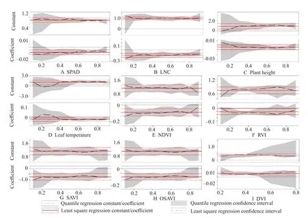
Fig. 3 Coefficients of intercept and slope given different quantiles

Results

Quantile regression model

Additional analyses were performed on the model using the preliminary classification criteria as discussed. Hypothesis testing results are presented in Fig. 4.

Hypothesis test results for nine quartile regression models (Fig. 4) showed thatP-values for the first kind that encompassed plant height and leaf temperature as independent variables were all higher than 0.05,given any quartile. These results were not statistically significant, but significant correlations were obtained among plant height, leaf temperature and rice yield.

The quantile regression model established using SAPD as the independent variable exhibited significant regression given quantileτ≥0.3; on this basis,the estimated model coefficient value was between-0.01154 and -0.00557. All the three models performed well overall. The quantile regression model that used SAVI and OSAVI as independent variables yielded an estimated range of coefficients within the range (-1.05185, 0.6307) and (-1.31039, 0.96769),respectively. This model exhibited high signi ficance at almost all the quantiles. Indeed, just atτ=0.2, the two models assumed thatP-value of the test results was greater than 0.05. The quantile regression model built using NDVI as the independent variable generated estimated values of its coefficient term between-1.49374 and -0.24152, including a signi ficant quantile segment within the range (0.1, 0.8).

Slopes (i.e., the estimated coefficient term) of the regression line at each model quantile evaluated by using the hypothesis test were not the same(Table 3).

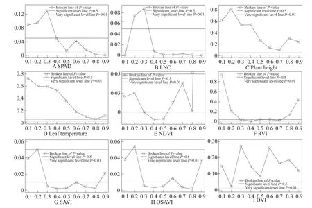
Fig. 4 Hypothesis test results for nine quantile regression models

Table 3 Regression line coefficients at different quantiles

The data presented in Table 3 showed that the regression line trend of quantiles for each predictive variable under different points remained the same.Indeed, in the case of SPAD variable, the slope of the regression line at each quantile was different, which reflected differences in the distribution of SPAD at each quantile.

Production estimation

The accuracy of the rice yield estimation model constructed here was evaluated based on rice growth parameters and vegetation indices at the jointing stage.Validation was performed on the basis of independent test data obtained from Hulan District Experimental Field (Heilongjiang, China) in the same year (n=12)with root mean square error (RMSE) and mean absolute percentage error (MAPE) used as test indices.RMSE and MAPE were derived for prediction values on the basis of equations (8) and (9), respectively(Table 4). Sample number measured and estimated yield values were included in the model. This meant that values of RMSE and MAPE represented the distance between the estimated and the true values, as the followings:

Table 4 Accuracy evaluation model for rice yield estimation

Verification results showed that MAPE value for the quantile regression model was lower than that recovered for OLS regression model (Table 4). As it was influenced by outliers, RMSE values of the quantile regression model including SPAD as the independent variable were slightly higher, while those for the former or for other quantile regression models were all lower than those of OLS regression values.Indeed, as RMSE used average error which was also sensitive to outliers and because the ratio between error and real value (MAPE) needed to be considered,it was clear that the overall accuracy of the quantile regression model per unit yield estimation was higher than that in other approach. MAPE values (5.107 and 5.528) for models constructed using RVI and DVI as input variables were also significantly higher than the average level of other vegetation index variable models (less than 5).

Discussion

In the case of the dependent variable (high yield level) at the middle and high ends of the conditional distribution, the influence of SPAD was higher than the average, while in the case of the dependent variable (low yield level) at the middle and low ends of the conditional distribution, the influence of SPAD remained relatively low. The effect of LNC on rice yield per unit was similar to that of SPAD in this case.This analysis revealed the presence of a close linear relationship among rice yields, SPAD and LNC under high yield per unit conditions. Fewer quantiles were available for selection in the case of RVI variable.In this case, the slope of the line at middle and low scores (τ=0.3, 0.4) was higher than that at middle and high scores (τ=0.6, 0.7), while DVI variable was only returned significantly within the low quantileτ=0.2.

In terms of NDVI variable, the effect on the yield per unit area of the dependent variable was mainly concentrated at both ends of the conditional quantile.This outcome included a large marginal contribution;its quantile regression line reached maximum slope atτ=0.7. This result could be used to construct a quantile regression model at high yield level. Indeed,for variables SAVI and OSAVI, with the exception of quantilesτ=0.1 andτ=0.2, the effects of the model on the distribution of yield per unit area of the dependent variables remained relatively consistent. The linear relationship between variables SAVI and OSAVI versus the dependent variable yield per unit yield remained close, given normal rice yields; the slope of the regression line reached a maximum value atτ=0.6.

Conclusions

The regression results and test indices of the quantile regression model and OLS regression model were compared and analyzed. There was a number of clear conclusions that resulted from this work. First, the precision of the quantile regression yield estimation model was better than that of OLS regression yield estimation model. This quantile regression was not sensitive to outliers. The established production estimation model was more robust and more accurate and it provided a bene ficial supplement to the general regression. Second, the quantile regression model encompassed a detailed and comprehensive description of the dependent variables with different conditional distributions. On the basis of this characteristic, the quantile regression model underτ=0.7 of NDVI and generated rice yield per unit area under quantile was determined to build an optimal estimation model.