Learning material law from displacement fields by artificial neural network

Hang Yang, Qian Xiang, Shan Tang,*, Xu Guo,*

a State Key Laboratory of Structural Analysis for Industrial Equipment, Department of Engineering Mechanics, Dalian University of Technology, Dalian 116023, China

b International Research Center for Computational Mechanics, Dalian University of Technology, Dalian 116023, China

Keywords:Data-driven Material law Displacement field Digital image correlation Artificial neural network

ABSTRACT The recently developed data-driven approach can establish the material law for nonlinear elastic composite materials (especially newly developed materials) by the generated stress-strain data under different loading paths (Computational Mechanics, 2019). Generally, the displacement (or strain) fields can be obtained relatively easier using digital image correlation (DIC) technique experimentally, but the stress field is hard to be measured. This situation limits the applicability of the proposed data-driven approach. In this paper, a method based on artificial neural network(ANN) to identify stress fields and further obtain the material law of nonlinear elastic materials is presented, which can make the proposed data-driven approach more practical. A numerical example is given to prove the validity of the method. The limitations of the proposed approach are also discussed.

Materials law plays a key role in mechanics problems as it can relate strain to stress response for a given material. Although many function-based material models are proposed, it is difficult to cover all the materials especially for some newly developed materials. Building an appropriate material law usually requires long-time efforts through the traditional approach,which severely inhibit the use of the newly developed materials in engineering design.

Recently, many data-driven approaches are proposed, which can replace the function-based material law with data. For example, Kirchdoerfer and Ortiz [1] solved the boundary-value problems in mechanics by minimizing the distance of both computed stress and strain to the stress–strain database of a material. A self-consistent clustering analysis (SCA) was also proposed to reduce the computational cost in Liu’s group [2–4]. Our previous works showed the possibility of replacing the materials law of composites by artificial neural network (ANN) trained by stress–strain data [5, 6]. In these approaches, the database of stress–strain data under different loading paths is pre-required.However, it is difficult to obtain a homogeneous stress-state under multi-axis loadings in the experiments. For inhomogeneous stress-states, the stress fields are hard to obtain directly. But the displacement fields can be measured by digital image correlation (DIC) technique relatively easier [7]. With the measured displacement field by DIC, the parameters involved in the existing function-based hyperelastic models such as Mooney–Rivlin can be calibrated [8–10]. Réthoré [11] further considered the identification of Poisson’s ratio based on the perturbed displacement fields by noises.

Despite the success of these model-based parameter-identification methods, integration the recognition of material law with the data-driven approach is very attractive because it can avoid the choice of the existing function-based material models or construction of a new one. A stress–strain database can be obtained through the experiments [12–15], which can be used to solve the boundary-value problem by the data-driven approach initialized by Ortiz’s group [1], avoiding the function-based material law.

In this paper, a data-driven method is proposed to identify the material law based on the measured displacement fields through ANN. The obtained material law based on ANN can be integrated seamlessly with our proposed data-driven approach to solve boundary value problem under the displacement-driven finite element framework. The learned material law is also very flexible to be integrated into commercial software or inhouse code and numerical solving shows the second-order convergence [5].

The force balance method (FEMU-F) [16–18], which can obtain the parameters in the existing function-based material law based on the available displacements of all the nodesin the experiments, is further developed in this paper. In combination with ANN, it is possible to build a material law without any explicit functional form, which is described in the following. All subsequent formulations are consistent with the current DIC technique under the plane stress conditions.

The left Cauchy–Green tensor and the Cauchy stress are chosen as measures of strain and stress because they are coaxial under the isotropic assumption. The left Cauchy–Green tensor is defined as

where F is deformation gradient, given by F =I+. Here, I and ∇0are the second-order identity tensor and the gradient operator defined in the original configuration, respectively. The Cauchy stress σ can be given through an implicit function ϕ as Here the ANN can play the role of this function. In the proposed approach, the function ϕ rotates the input b first to the principal direction. Then the two principal components of b (b1and b2)are input into the ANN with the different order (b1and b2are switched) (see the upper and lower ANNs in Fig. 1. The two ANNs share the same weights and bias, which can be considered to be the same ANN actually.) The adoption of the two ANN is to ensure that the materials law is strictly isotropic [5]. Finally the outputs of the ANN are averaged and rotated back to the original directions. This process of computing σ from b is shown in Fig. 1,and summarized in the following:

• Compute the eigenvalues and eigenvectors of b:

where biand Nirepresent the eigenvalues (principal component) and eigenvectors of b, respectively.

• Compute the principal stress by ANN:

where w and β are the wight and bias of the ANN (fANN),represents the i-th output of the ANN, and σirepresents the i-th principal component of σ. More details about the ANN are given in the appendix.

• Compute the stress in the original directions:

The internal force of each nodecan be predicted through finite element method (FEM) as

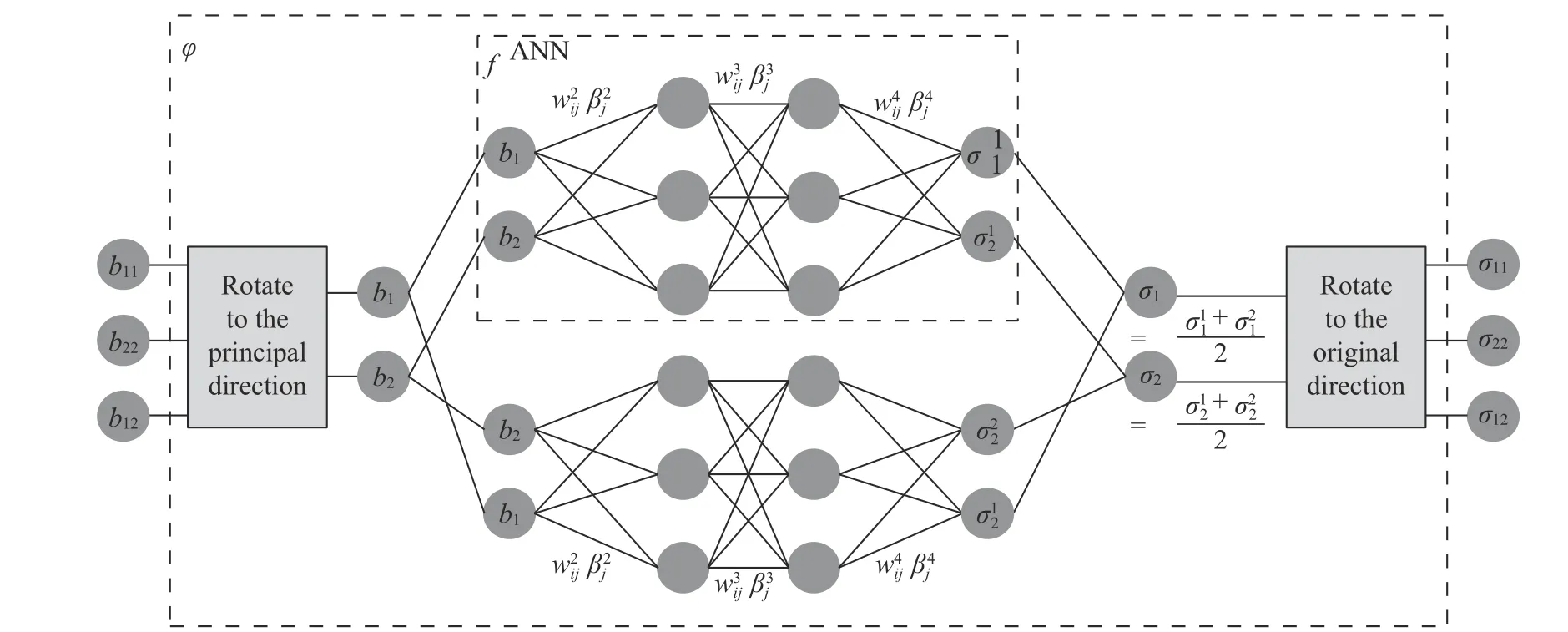
Fig. 1. Artificial neural network for strictly isotropic nonlinear elastic materials. The dotted boxes identify the functions of ϕ and f ANN defined in the paper. The weights w and biases β and its components and are also marked. The mapping from the left Cauchy-Green tensor to the Cauchy stress can be obtained after ANN training.

which is a function of w and β. Here Ω(e)is the area of the element e, and B(e)is strain-displacement matrix depending on the shape function [19]. The total force on all the nodes should also satisfy the equilibrium condition, which can be written as follows

where Ω represents the internal area and Sσrepresents the boundary with the externally imposed force fext. Equilibrium equations can be transformed into a minimization problem as

where viis the introduced weight greater than zero which can improve the convergence to the global optimal solution. Two regularization terms for both weights and bias are also introduced to prevent over-fitting, and the optimization should be carried out in the entire loading process as

where T is the total time of the loading process, λ is the regularization coefficient, ∥ ·∥L2is L2 norm operator, and (·)(t)is the value of (·) at time t. This is a non-convex unconstrained optimization problem, which can be solved by intelligent optimization algorithm (e.g., particle swarm optimization) or stochastic gradient descent method (the gradients can be obtained by back propagation algorithm of ANN).

The solving process is similar to the standard ANN training,discussed in our previous work [5]. The difference is that the entire process only provides input data (the measured displacements), and the output data (stress) is not required and replaced by the equilibrium condition. The ANN does not compute the node forces directly, but predicts the stress in each element. The force on a node is computed by the stress from multiple elements, and the stress of an element also affects the node force of multiple nodes, explained in Fig. 2. It can be seen that elements 1, 2, and 4 jointly determine the force of the blue node that needs to be in equilibrium with the external force. Elements 1, 3, 4, 5, 6 and 7 jointly determine the force of the red node that needs to reach the zero resultant force. At least one non-zero force boundary condition is required. Otherwise it converges to the solution with all-zeros.

The optimization problem discussed above is not a convex one, so the ordinary gradient-based optimization method usually is hard to give the globally optimal solution. It tends to converge to a solution where the weights w and biases β are all-zeros, leading to the predicted stress with zeros. In this situation,only the equilibrium condition on the boundary with the externally imposed force cannot be satisfied but all other nodes can,which is a local optimal solution. The situation can be improved by increasing the weight viof nodes on the boundary in Eqs. (8)and (9). On the other hand, intelligent optimization algorithms can solve this problem well. The cost of computation is much lower than that of the sample preparation and physical experiments.

The displacement fields used to learn the material law must contain enough multi-axis stress-states so that the trained ANN can predict the stress accurately with arbitrary strain. Otherwise,the trained ANN cannot predict the mechanical responses under some specific stress-states. The gathering of the measured displacement fields from different specimens can be used to train the ANN together to avoid this issue. More detailed discussion is given as below.

The proposed method shown in the above only considers the two dimensional problem (plane stress), which can be naturally extended to three dimension problem. But the method is limited by the DIC technology, which can only measure the displacement/strain on the 2D surface.

A rectangular plate with three circular holes of different radius under the imposed tensile loading is investigated under plane stress conditions. The unit of length is mm; force is N; stress,pressure and modulus are MPa. The geometric setup is shown in Fig. 3a. Six equally spaced concentrated forces are applied to the right edge. On the left edge, both X and Y degrees of freedom are fixed. The Ogden model with parameters µ = 5, α = 2, and D =0.01 is employed (the definition of these parameters is consistent with ABAQUS manual). The displacement field is computed by FEM with the given Odgen model. The entire loading process is equally divided into 6 incremental steps. Particle swarm algorithm, in which the swarm size is 1000, is used to solve the optimization problem (Eq. (9)), identifying the weights w and biases β of the ANN. Note that the numerical experiment is used to replace the role of DIC technique to obtain the required displacement fields for the optimization problem. The employed ANN consists of two hidden layers with 3, 3 neurons respectively.

The predicted stress fields by both the reference and the trained ANN models are plotted in Fig. 3(c, d). Define the relative error of the effective stress between two models as

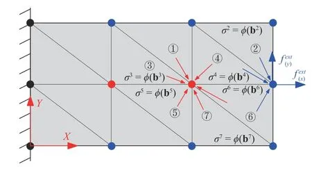
Fig. 2. Physical explanation of equilibrium equations by ANN model. The nodes are marked blue on the boundary with the externally imposed force, black on the boundary with the imposed displacement and red inside the simulated domain. The internal force is equal to the external force on the blue nodes, and equal to zeros on the red nodes. The force on the black nodes are not considered. The force on each node depends on the stress of all the elements that contain the node, and each element has an effect on the force of all the nodes belonging to it.

The principal components of the left Cauchy–Green tensor,b1and b2in all the elements of the numerical example during the whole loading process are summarized in Fig. 5. The ANN trained model by the given displacement fields can accurately predict the stress when the strain is close to the data points shown in the figure, but it cannot predict stress accurately when the strain is far from the data points. Most points lie in the II and IV regions while only a few in the I and III regions. In order to predict mechanical response better, the displacement field reflecting the deformation modes shown in the I and III region should be introduced to train the ANN together.

In this paper, a data-driven method based on ANN to obtain the material law is proposed. The proposed method can be used to quickly build the material law for isotropic nonlinear elastic materials based on the measured displacements in the experiments. In this short paper, the displacement field is generated by the numerical experiments rather than the DIC measurement. If the data of the displacement fields measured by DIC is used, the same way can be used.

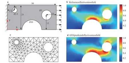
Fig. 3. Numerical example for a rectangular plate with three holes. a Geometric model and boundary conditions of the voided plate. The contour plots of effective stress computed by b the finite element simulation with the reference Odgen model and d the proposed method. c Finite element mesh contains 142 nodes and 226 element.

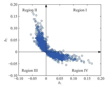
Fig. 5. Summary of all the strain states during the loading process.The principal components of the left Cauchy-Green tensor, b1 and b2 of every element at each time step are plotted.

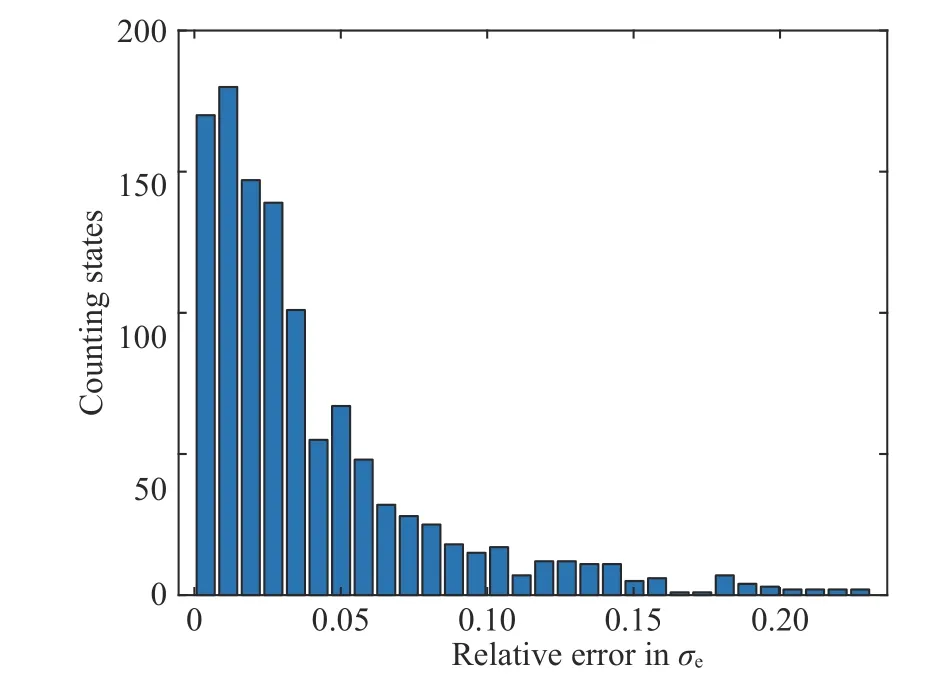
Fig. 4. Statistics of the relative error between the predicted results by the proposed method and the reference Odgen model. The results of all incremental steps are counted together.

The proposed method can only be applied to isotropic nonlinear elastic materials at present. In the future, it should be extended for more complex materials such as elastoplastic and viscoelastic materials. Numerical techniques for improving efficiency and robustness of the proposed method should also be incorporated. These things leave abundant room to improve the present method.

Acknowledgement

S. Tang appreciates the support from the National Natural Science Foundation of China (Grant 11872139). X. Guo thanks the support from the National Natural Science Foundation of China (Grants 11732004 and 11821202), and Program for Changjiang Scholars, Innovative Research Team in University(PCSIRT).

Appendix: Discussion on the ANN

ANN is briefly discussed here. The reader can refer to our previous work for more details [5]. For a general ANN, a functional transformation is defined as

on n-th layer (superscript n represents the layer number), which can map the data unit on i-th neuronfrom the n-th layer to (n+1)-th layer, whereis the weights for the link between i-th neuron on n-th layer and j-th neuron on (n+1)-th layer, andis the bias for the j-th neuron on (n+1)-th layer.

For materials law described in the principal directions, the iteration for ANN training starts from the input layer with the principal component of the left Cauchy–Green tensor as the input:

which correspond to the upper and the lower ANNs in Fig. 1,respectively. The two ANNs share the same weights and bias.The mapping from n-th layer to (n+1)-th layer takes

The outputs at the final layer are the principal components of the Cauchy stress in Eq. (4) as

where N represents the total number of layers of the ANN.