Classifying wakes produced by self-propelled fish-like swimmers using neural networks

Binglin Li, Xiang Zhang, Xing Zhang,*

a State Key Laboratory of Nonlinear Mechanics, Institute of Mechanics, Chinese Academy of Sciences, Beijing 100190, China

b School of Engineering Science, University of Chinese Academy of Sciences, Beijing 100049, China

Keywords:Flow sensing Machine learning Wake classification Self-propelled swimming Fluid-structure interaction

ABSTRACT We consider the classification of wake structures produced by self-propelled fish-like swimmers based on local measurements of flow variables. This problem is inspired by the extraordinary capability of animal swimmers in perceiving their hydrodynamic environments under dark condition. We train different neural networks to classify wake structures by using the streamwise velocity component, the crosswise velocity component, the vorticity and the combination of three flow variables, respectively. It is found that the neural networks trained using the two velocity components perform well in identifying the wake types, whereas the neural network trained using the vorticity suffers from a high rate of misclassification. When the neural network is trained using the combination of all three flow variables, a remarkably high accuracy in wake classification can be achieved. The results of this study can be helpful to the design of flow sensory systems in robotic underwater vehicles.

The long-lasting wake structures left behind active swimmers and inanimate objects contain useful hydrodynamic cues about the sources that produce them. Such information can be extracted and exploited by other swimmers to accomplish a variety of tasks [1]. For example, with the help of the lateral line system, even blind fish can school [2] and avoid obstacles in the water [3, 4]. By using the whiskers, harbor seals can track the preys by detecting the wake signals [5]. This remarkable capability in animal swimmers also inspired the development of artificial flow sensory systems [6–10].

The wake structures behind a bluff body and an active swimmer are often characterized by the von Karman and reverse von Karman vortex streets, respectively. Based on the number of vortices that are shed per flapping cycle, the wakes produced by an active swimmer can also be further classified into different subtypes. The “2S” and “2P” wakes are the two most commonly seen sub-types. Here “2S” refers to the situation in which two vortices of opposite sign are shed per cycle; whereas “2P” refers to the situation in which two pairs of vortices are shed per cycle. Besides, some higher-order exotic wakes, with up to 16 vortices shed per cycle have also been observed [11]. The types of wake produced by the swimmers are intimately associated with the swimming characteristics.

For an animal (or artificial) swimmer, the capability of distinguishing between different wake types lays the groundwork for motion planning and navigation. However, this seemingly easy task is actually an inverse problem which poses great challenges to the flow sensory system. The reason is that the data of measurements are only available at discrete locations within a small sub-domain of the entire flow field. This is in contrast with the situation faced by an outside observer to whom the globally spacial-temporal flow patterns are accessible.

With the rapid progress of machine learning, fundamental methodologies in machine learning have been used to handle the tasks of fluid mechanics [12]. Recently, some pioneering works have been conducted to solve this inverse problem by using machine learning algorithms. Wang and Hemati [13] generated “2S” and “2P” wakes with the point vortices by using the ideal-flow model. The wake-induced velocities were measured on the surface of a fish-like body that was immersed in the vortical wakes. The K-nearest neighbors (KNN) algorithm was then used to classify the wake types. Colvert et al. [14] generated the wakes behind a tethered rigid pitching foil placed in an otherwise steady stream by solving the Navier−Stokes equations numerically. The neural networks were then trained to distinguish between three distinct wake types from the time histories of vorticity measured at discrete locations. Alsalman et al. [15] used the same wakes as those generated by Colvert et al. [14], and went one step further to investigate how the accuracy of wake classification was affected by the types of sensors (i.e., sensors measuring different flow variables). They also trained the neural networks to classify wake types from the data of “one time”measurements at a spatially-distributed array of sensors. Motivated by the aforementioned studies, in this work, we train the neural networks to classify wakes behind a self-propelled fish-like swimmer. Similar to the studies of Refs. [14, 15], in the present study the wakes are also produced by high-fidelity numerical simulations. However, the wakes considered here and those in the two aforementioned works are very dissimilar, in terms of the spatial-temporal patterns. Clearly, the wakes considered here bear a much closer resemblance to those produced by an animal (or an artificial) swimmer under free-swimming condition.

We consider continuous and intermittent self-propelled swimming of a flexible fish-like swimmer which is driven by fluid-structure interaction (FSI) [16, 17]. The localised actuation consists of the coupled heaving and pitching motions that are imposed at the leading edge (see Fig. 1). For the continuous swimming, the driving motions are:

where ys=0and θs=0are the instantaneous heaving and pitching displacement of the leading edge; A and Aθare the heaving and pitching amplitudes, respectively; f is the actuation frequency,and ϕ is the phase lag between the heaving and pitching motions. In this study, the phase lag is set to 90°. For the intermittent swimming, certain time duration of passive coasting is interspersed between two half-periods of active bursting(flapping) [16]. The degree of intermittency is characterised by the duty cycle (DC), which is defined as the ratio of the time duration of active flapping to the time duration of one full cycle of burst-and-coast locomotion.

The incompressible Naiver−Stokes equations and nonlinear dynamics equations constitute the governing equations of the system. These equations can be written in a dimensionless form as:

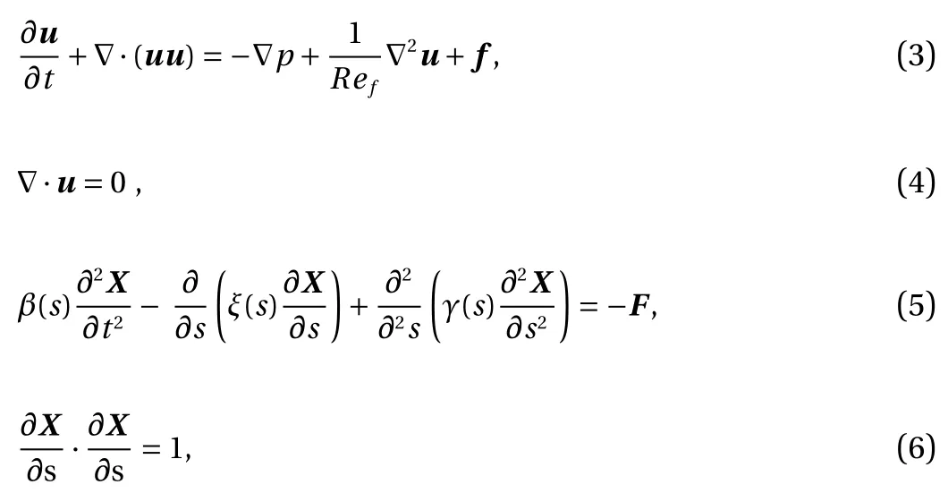
where u is the fluid velocity; p is the pressure; X is the position vector for the Lagrangian (marker) point on the flexible swimmer and s is the Lagrangian coordinate along the arc; f and F are the dimensionless Eulerian and Lagrangian forces which represent the interaction between the flow and the structure. We select the chord length L and Uref=L f as the reference length and reference velocity for scaling the system.The four dimensionless quantities that arise in the governing equations are: flapping Reynolds number Ref, mass ratio β,dimensionless tension ξ and dimensionless rigidity γ. The definitions of these four dimensionless quantities as:

Fig. 1. Schematic diagram of the wake classification problem: an array of sensors is placed in the wake behind a self-propelled fish-like swimmer.

where ν is the kinematic viscosity of the fluid; ρfand ρsare the densities of the fluid and the filament, respectively; δ is the thickness of the filament; T and B are the tension and bending ri gidity of the structure, respectively. Here ξ is a Lagrangian multiplier which is determined to enforce the inextensibility condition (Eq. (6)) [18]. β and γ are two exponential functions with respect to s [16, 17]. In this study, R efis fixed to 6 000, which is the same as the highest Reynolds number considered in Ref.[16]. The Reynolds numbers based on the swimming velocity lie in the range of 3000 to 4000. The coefficients in the two aforementioned exponential functions are tunable.

This FSI problem is simulated by using a loosely-coupled solver in which the flow equations and structure equations are advanced sequentially in time. In solving the flow equations, the immersed boundary method is used to impose the no-slip condition on the surface of the swimmer. In solving the structure equations, a finite difference method is used for the spatial discretization and a three-time-level scheme is used for the temporal advancement. This FSI solver has been extensively validated in the earlier works of our group [16–20]. After solving for the velocity field u (x,t), the scalar vorticity field is computed by ωz=(∇×u)·k , where k is the unit normal vector which points towards the “outside” of the two-dimensional plane. Here the second-order central-difference scheme is used to discretize the curl operator ( ∇×).

We conducted nine cases of simulation by tuning some control parameters. These parameters include: coefficients of the exponential functions that govern the distributions of β and γ,dimensionless heaving amplitude A /L , pitching amplitude Aθ,and duty cycle D C. Among all simulation cases, three distinct wake types, namely, “2S”, “2P”, “2P+2S”, are identified. The values of the control parameters and wake type corresponding to each simulation case are listed in Table 1. It is seen that each wake type can be observed in three different simulation cases.The representative vortex structures for the “2S”, “2P” and“2P+2S” wakes are shown in Fig. 2.

The wake detection zone is of rectangular shape and has the dimensions of 5 L×2L. It is symmetric with respect to the horizontal centerline and is placed downstream of the swimmer with a distance of L from the trailing edge. Unlike the previous studies in Refs. [14, 15], where the time histories of flow variables were used for wake classification, here we only use the data of“one time" measurements. The reasons for this choice in the present study are twofold. First, in the wake produced by a selfpropelled swimmer, “decaying with time” is the salient feature in the time histories of flow variables, while temporal periodicity does not show up in the signals. Second, the wake classification based on the data of “one time” measurements implies that there is no time delay. This is certainly more favorable in the design of flow sensory systems in animal (or artificial) swimmers. For each simulation case listed in Table 1, the data sampling frequency is 20 times per flapping cycle, and the duration of sampling is 5 flapping cycles. As a result, the data of 100 snapshots are collected. For each snapshot, the vorticity ( ωz) and two velocity components (uxand uy) at the grid points of the computational mesh are saved. Before later usage in training and testing the neural networks, all flow variables are preprocessed by scaling with the root-mean-square (RMS) values of the collected data.

A spatially distributed array of senors with the length of L is then used to measure the flow variables (see Fig. 1). The sensor array is in align with the x-axis and the number of sensors is set to 6. For each snapshot, the measurements are conducted 861 times, by placing the first (leftest) sensor on the vertices of a 41×21 lattice which occupies part of the detection zone. The vertices of the lattice are uniformly distributed and the interspace between two neighboring vertices is 0 .1L. Thus, for each simulation case, 861 × 20 × 5 = 86100 measurements are conducted by the sensor array. Since the positions of sensors are not necessarily in coincidence with the positions of grid points, bilinear interpolations are performed to obtain the values of flow variables at the positions of sensors.

We train fully connected neural networks (FCNs) to classify the wake structures. The hyperparameters of the neural networks are listed in Table 2. Specifically, the FCNs consist of 3 hidden layers and 1 output layer and each hidden layer has 32 units (neurons). We test the effects of the numbers of hidden layers and units on the performance of the networks. It is found that the networks exhibit little variation in performance if the number of hidden layers or the number of units is further increased.The output of each unit is the input of ReLU activation function.The output layer is a softmax function which can map the output of the last hidden layer to a probability distribution vector.This vector has three components which indicate the probability of the three predicted wake types. Thus, the values of thethree components lie in the range of 0 to 1. The loss function of the FCNs is the cross-entropy function which can be written as:

Table 1 Control parameters of the fish-like swimmers used to produce the wakes.

where pi(x) is the true probability distribution vector by using one-hot encoding that identifies the wake type and qi(x) is the predicted distribution vector obtained from the FCNs. The training of the FCNs is performed by minimizing the loss function to approach the real distribution of the target. In this work, the neural networks are implemented using the open source machine learning package TensorFlow.

The FCNs are trained and tested by using the approach of three-fold cross-validation. More specifically, for each wake type, the measurement data obtained from two simulation cases are used for training and the data from the remaining case is reserved for testing. Altogether, three distinct data sets (Data set 1,Data set 2 and Data set 3) are created by different combinations of the simulation cases for training and testing (see Table 3).

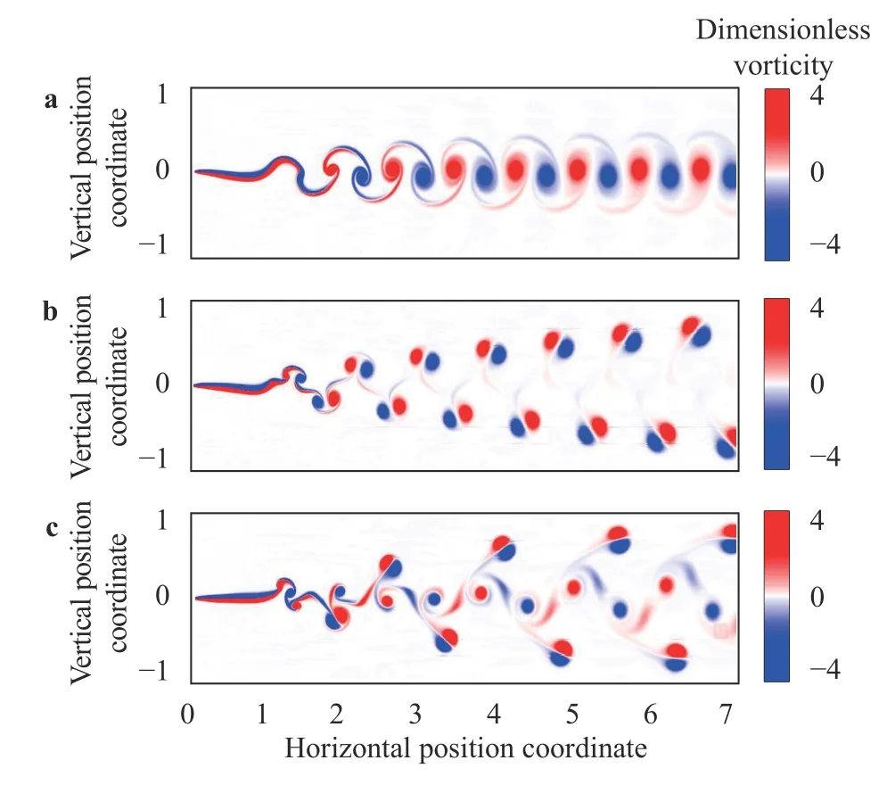
Fig. 2. Representative vortex structures for the three types of wake:a “2S” type; b “2P” type; c “2P+2S” type. The vortex structures are visualized using the contours of dimensionless vorticity (vorticity scaled by f).

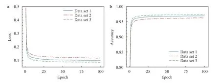
Fig. 3. Values of loss function and network accuracy versus the number of training epochs in training the FCN using the combination of all three flow variables: a loss function; b network accuracy.

Four types of FCNs are trained using the measurements of different flow variables as the input data. The first three FCNs are trained by using ux, uyand ωz, respectively, while the fourth FCN is trained by using the combination of all three flow variables. In Fig. 3, we show the progress to convergence in training the FCN using all three flow variables as the input. It is seen that 100 epochs are sufficient for the network to reach its best performance, since both the loss function and accuracy exhibit little variation with the increase of epoch number. Similar behaviors are also observed in the training of other three FCNs (the progress to convergence for them are not shown here for brevity).

We then evaluate the performances of the four FCNs in classifying the wake structures. The performances of the FCNs are visualized using the normalized confusion matrices. The definition of confusion matrix is as follows. Each row of the confusion matrix represents the instances in an actual class, while each column represents the instances in a predicted class. Thus, the diagonal and off-diagonal entries of the matrix show the instances of correct classification and misclassification, respectively. A normalized confusion matrix is constructed by normalizing the entries of each row of the confusion matrix using the total instances in the actual class (i.e., the summation of all entries in that row). The normalized confusion matrices for the three FCNs trained by using ux, uyand ωzare shown in Fig. 4. The ac-curacies shown in the normalized confusion matrices are the averaged results obtained by using three different data sets. It is seen that the FCN trained using uxperforms very well. For all three wake types, the percentage of correct identification are higher than 9 0%. For the “2S” wake, the rate of correct identification can even reach 9 8.3%. The FCN trained by using uyperforms comparably with the FCN trained using ux. For these two FCNs, the highest rate of misclassification is around 6 % to 7 %.The performance of the FCN trained using ωzis much worse. In identifying the “2S”, ”2P” and “2P+2S” wakes, the percentages of misclassification are 6.1%, 58.6%, and 24.4%, respectively.

Table 2 Hyperparameters of the FCNs used in the wake classification.

Table 3 Different combinations of simulation cases in the threefold cross-validation for training and testing the neural networks.

Fig. 4. Normalized confusion matrices for the three FCNs trained using a ux; b uy; c ωz.

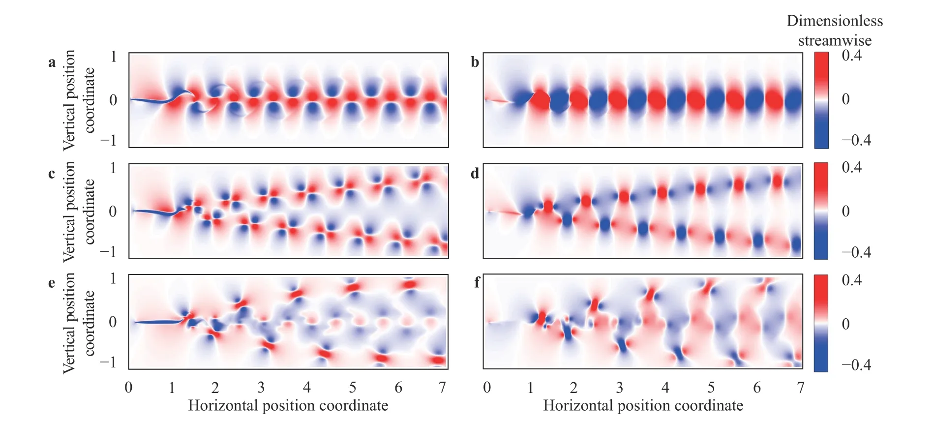
Fig. 5. Contours of the two velocity components in the “2S”, “2P” and “2P+2S” wakes. a and b (dimensionless) streamwise and crosswise velocity components for the “2S” wake; c and d (dimensionless) streamwise and crosswise velocity components for the “2P” wake; e and f (dimensionless) streamwise and crosswise velocity components for the “2P+2S” wake.

The poor performance of the FCN trained using ωz(especially in identifying the “2P” wakes) can be explained as follows.By examining the vorticity contours shown in Fig. 2, it is seen that for the “2P” wake, in a large portion of the wake detection zone, the vorticity magnitude is very small (close to zero). This makes it very difficult for the FCN to extract the intrinsic feature of the wake from local measurements of ωz. In contrast with the contours of ωz, the contours of uxand uylook very different (see Fig. 5). It is seen that the contours with high magnitudes of uxand uyare less concentratedly distributed in the wake detection zone. This makes it easy for the FCNs to uncover the salient feature of each wake type.ux, uyand ωz) as the input data. It is seen that remarkably high Figure 6 shows the normalized confusion matrix for the FCN trained by using the combination of all three flow variables (i.e.,accuracies in identifying all three wake types have been achieved. The highest rate of misclassification is reduced to 3%(which is observed in identifying the “2P+2S” wakes). The superior performance of the FCN trained using all three variables can be explained as follows. The spatial distributions of the three flow variables measured by the sensor array can complement each other and result in reduction of confusion among the three wake types.

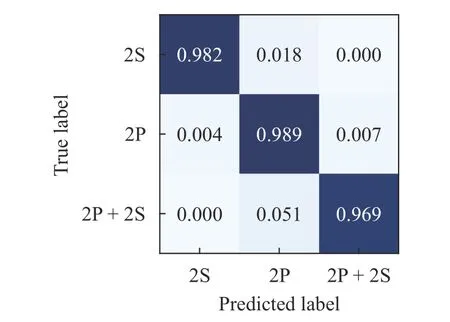
Fig. 6. Normalized confusion matrix for the FCN trained using the combination of ux, uy and z.

In this work, we trained four types of FCNs to distinguish among three types of wakes produced by a self-propelled fishlike swimmer. We used the “one time” measurements of some flow variables (including the two velocity components and the vorticity) as the input data in training the neural networks. It turned out that the FCN trained using streamwise or crosswise component of velocity performs much better than the FCN trained using vorticity. The FCN trained by using the combination of all three flow variables outperforms the other three FCNs and achieves a remarkably high accuracy in wake classification.

There are a number of interesting avenues for future research. First, the sensitivity of the performance of the neural networks to the number and arrangement of sensors needs to be studied. Second, the neural networks can be used to discern more useful information of the swimmer from the wake, such as the body size, species, swimming speed and swimming style.This is achievable only if a solid link between such information and the localized flow measurements can be established. Third,one limit of the current study is the assumption that the placement of sensors in the detection zone does not disturb the flow.The two-way interactions between the sensors and the flow need to be considered.

Acknowledgement

This work was supported by the National Natural Science Foundation of China (Grants 11772338 and 11372331), Chinese Academy of Sciences (Grants XDB22040104 and XDA22040203).