Summed volume region selection based three-dimensional automatic target recognition for airborne LIDAR
2020-06-28QishuQianYihuaHuNanxiangZhaoMinleLiFucaiShao
Qi-shu Qian , Yi-hua Hu ,*, Nan-xiang Zhao , Min-le Li , Fu-cai Shao c
a State Key Laboratory of Pulsed Power Laser Technology, National University of Defense Technology, Hefei, 230037, China
b Anhui Province Key Laboratory of Electronic Restriction, National University of Defense Technology, Hefei, 230037, China
c The Military Representative Bureau of the Ministry of Equipment Development of the Central Military Commission in Beijing, Beijing,100191, China
Keywords:3D automatic target recognition Point cloud LIDAR Airborne Global feature descriptor
ABSTRACT Airborne LIDAR can flexibly obtain point cloud data with three-dimensional structural information,which can improve its effectiveness of automatic target recognition in the complex environment.Compared with 2D information, 3D information performs better in separating objects and background.However, an aircraft platform can have a negative influence on LIDAR obtained data because of various flight attitudes, flight heights and atmospheric disturbances. A structure of global feature based 3D automatic target recognition method for airborne LIDAR is proposed,which is composed of offline phase and online phase. The performance of four global feature descriptors is compared. Considering the summed volume region(SVR)discrepancy in real objects,SVR selection is added into the pre-processing operations to eliminate mismatching clusters compared with the interested target. Highly reliable simulated data are obtained under various sensor’s altitudes, detection distances and atmospheric disturbances. The final experiments results show that the added step increases the recognition rate by above 2.4% and decreases the execution time by about 33%.
1. Introduction
With the development of LIDAR, extending automatic target recognition(ATR)from the 2D to the 3D domain becomes possible and more attractive.3D data can indicate the structure of an object and lessen the effect of illumination variation and object altitude changes. Current 3D ATR algorithms mainly operate in automatic drive domain and have already been put into real-time use [1].Switching the LIDAR platform from cars to aircrafts can offer a topdown view to reduce the horizontal occlusion of objects on the ground. Except from the practical use of ATR in the battlefield,close-range LIDAR scans can be easily spotted.Airborne LIDAR can work in a long range and decrease risks from long-time exposure on the region.
ATR algorithms can be divided into local and global feature descriptors based algorithms.Kechagias-Stamatics[2]evaluated 3D local descriptors and proposed an ATR structure [3] that used signature of histograms of orientations(SHOT)descriptor[4].Local feature descriptors, as SHOT, rotational projection statistics (RoPS)[5],3D shape context(3DSC)[6],and fast point feature histograms(FPFH)[7],usually represent geometrical information around a key point. It is suitable to describe dense point clouds. However, with the same laser scanning resolution,fewer points are obtained from an object in a longer LIDAR-target distance, which decreases the performance of local feature descriptors. Global feature based descriptors will suit the above situation better for describing multiple information of a whole object.Many good global feature descriptors have been proposed,such as viewpoint feature histogram(VFH)[8],clustered viewpoint feature histogram (CVFH) [9], global radiusbased descriptor (GRSD) [10], ensemble of shape functions (ESF)[11], slice images [12] and geometric moments [13].
Appealed by the advantages of 3D features, we propose an airborne 3D ATR structure based on global feature descriptors,containing an offline phase and an online phase. The former is to train a template and feature base with single models generated under multiple viewing angles and LIDAR-target ranges. The datasets used are simulated but highly credible top-down view models and scenarios. The maximum LIDAR-target range in the current literature is set to 200 m,which is quite different from the actual situation. We extend the range to as far as 1800 m to make the simulation more practical. The latter phase, i.e. online phase,consists of object segmentation,the summed volume region(SVR)selection,feature extraction and feature matching.Considering that real-world object differs itself from the other in size, we add the SVR selection before feature extraction, excluding clusters whose spot sizes are too big or small compared with our interested targets.
The paper is organized as follows: In Section 2, an airborne 3D ATR structure is proposed.Then,in Section 2.1 and Section 2.2,the offline phase, the online phase, basic principles of method used in the pipeline and SVR selection are proposed. In Section 3, our pipeline on three highly reliable and challenging scenes from airborne platform is evaluated and three experiments of recognition rate and execution time are calculated. Finally, in Section 4,conclusions from the previous experiments are drawn.
2. 3D ATR structure for laser point cloud
The whole structure is show in Fig.1, which is divided into an offline phase and an online phase.In the offline phase,object point clouds are patched in various flight pitch, yaw angles and LIDARtarget ranges. Then, global feature descriptors and SVRs are computed. SVR can reflect the actual sizes of objects. Results are stored in Fast Library for Approximate Nearest Neighbors (FLANN)[14]. In the online phase, data pre-processing is used to filter the smooth surfaces in the scene and split the entire non-ground spots into separate clusters.SVR selection is to eliminate clusters that fail to reach the threshold.The reserved clusters are described by global descriptors.Finally,feature matching is done between the selected clusters and data built in the offline phase. It should be noted that the difference between our proposed structure and the one in Ref.[1]is that the use of global feature based descriptors can make ATR free of the post-processing phase.
2.1. Offline phase
2.1.1. Model and scenario generation
Single model and scenario data are acquired by simulating the working process of LIDAR because there are no open accesses for airborne LIDAR data at different flight heights. The global feature descriptors are trained for the potential military targets as tanks and planes. In the simulation process, six altitudes and LIDARtarget distances are set to make the simulation more credible.Fig. 2(a-f) shows the influence of three different distances on the scenes and the single M1 Abrams model. With the LIDAR-target distance becomes closer, the field-of-view becomes smaller and the number of points grows.The aircraft’s altitude changes will lead to changes of the space distribution of points. Fig. 2(f-i) shows point cloud data of a single tank model under four partial views.
Three types of scenes are airport,mountain and city scenes,and the specific information of each scene is shown in Table 1.
Compared to Refs. [1,2,19], our scenarios are more realistic and challenging since they are affected by a greater number of parameters. The course of the LIDAR seeking to the target is continuous.We set the farthest LIDAR-target range as 1.8 km,the nearest range as 0.3 km, and data are acquired at an interval of 0.3 km. At this point, the range resolution of the LIDAR increases from 1.8 km to 0.3 km.The experimental part includes the target recognition at six different sizes in three scenes, the change of target recognition accuracy before and after the application of SVR selection, and the robustness of the descriptor used in this paper to Gaussian noise of three intensities.
2.1.2. Feature extraction
Global feature descriptors are retrieved after obtaining point clouds at various aircraft altitudes and LIDAR-target ranges. In the offline phase, global feature descriptors are applied to 3D models that are built in advance. The range-pitch-yaw of the LIDAR-target is shown in Table 1. The global surface feature description is to encode surface geometrical information of entire 3D objects into a feature vector.Four global descriptors are selected for comparison.Suppose the point cloud P{P1(x1,y1,z1),P2(x2,y2,z2), …,Pn(xn,yn,zn)}to be computed.
VFH: It is made up by two parts: a viewpoint direction component,and an angular component with 3 angular features,α,φ and θ in 3 histograms.The object’s centroids found first.Then,the vector between the viewpoint (the position of the sensor) and centroid is computed, and normalized.Finally, for all points in the cluster, the angle between this vector and their normal is calculated, and the result is binned into a histogram. The vector is translated to each point when computing the angle because it makes the descriptor scale invariant. The second component is to compute the angular relationship for the centroid and its neighbors.
CVFH: It was introduced because the original VFH is not robust to the object cluster with missing points. To compute CVFH, the object is firstly segmented into several regions using regiongrowing method, and then a VFH is computed for every region.Thanks to this,an object can be found in a scene,as long as at least one of its regions is fully visible.
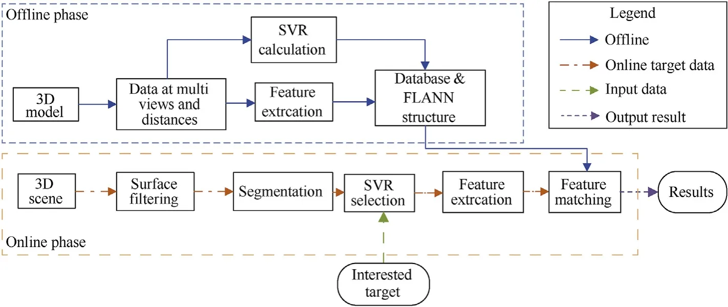
Fig.1. Airborne 3D ATR structure based on global feature descriptors.
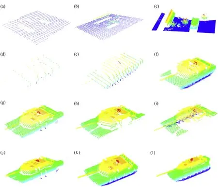
Fig. 2. The visualization of models under different conditions, (a) (d) 1800 m, (b) (e) 900 m and (c) (f) 300 m. When the platform is at pitch30°yaw:0°, (g-l) are under the 300 m LIDAR-target distance when the platform is at (g) pitch:60°yaw:0°(h) pitch:60°yaw:90°(i)pitch:60°yaw:180°(j) pitch:15°yaw:0°(k) pitch30°yaw:0°(l) pitch:45°yaw:0°.

Table 1 Parameters of three scenarios.

Table 2 3D feature descriptors evaluated.
GRSD: GRSD need voxelization and surface categorization step beforehand,labeling all surface patches according to the geometric category (plane,cylinder,edge,rim and sphere),using the Radiusbased Surface Descriptor(RSD).The radial relationship of the point and its neighborhood is computed. Then, the whole cluster is classified into one of these categories, and the GRSD descriptor is computed from this.
ESF: ESF combines three different shape functions which are respectively related with distances, angles and area of the points patched. Compared with other global counterparts, extracting ESF can be free of normal estimation. Besides, ESF is more robust to noise and partial points. This algorithm iterates through all the points. For each iteration, 3 points, {Pr1, Pr2, Pr3}, are randomly chosen from P.Then the shape functions D2,D2ratio,D3and A3are computed for these points.
2.2. Online phase
The input of the online part is the real-time data acquired by LIDAR and the interested target.After data pre-processing, feature extraction and matching are carried out to finally identify the target in the real-time scene.
2.2.1. Surface filtering
In order to improve the computational efficiency of subsequent feature extraction and matching, considering that the interested objects are usually non-ground parts of the scene, the surface filtering [15] is carried out first to extract non-ground parts. Secondly, extracted points are segmented into separate clusters to pave the way for subsequent feature extraction.
In this paper, cloth simulation [16] is used to segment ground points and non-ground points. The cloth model simulated by the particle spring model [17] is a grid composed of numerous interconnected nodes. Points are connected with each other by virtual springs and conform to the law of elasticity.After the cloth point is subjected to the external force,the change of it is linearly related to the force magnitude and this will produce a displacement. To get the shape of the cloth at a certain moment,the cloth point position in the 3D space needs to be calculated. According to Newton’s second law, the relation between the cloth point position and the interaction force is as Eq. (1).

Where,m is the mass of the cloth point, set as constant 1;X is the node position at a certain moment; Δt is the time step; G is the gravitational constant.
2.2.2. Object segmentation
Considering the running time of the algorithm, euclidean distance clustering algorithm is adopted for segmentation, and the range resolution of the real-time aircraft field of view is taken as the radius for search, and the non-ground points are divided into independent individuals. Firstly, Pi0is chosen, then, n points Pin}with the nearest distance to Pi0are obtained.

If the dPi0Pikis smaller than threshold, Pikwill be put into the assemble Q.The above steps will repeat until the number of points in Q reaches the maximum set in advance.
2.2.3. SVR selection
For the interested target,the number of points patched by LIDAR in certain LIDAR-target distance and angle has a certain scope according to its actual size. Considering that clusters segmented in Section 2.2.2 usually have different patched point numbers,the SVR selection is added in the pre-processing to lessen the following calculation and improve the total execution speed.
We extend SAT(Summed Area Table)from the 2D domain to the 3D domain as SVR. SVR is calculated as Eq. (3).

In Fig.3,SVR values of six kinds of objects in the 0.3 km,0.9 km,1.8 km LIDAR-target distance are shown.
Then, comparison is carried out with the threshold set in advance to decide whether the cluster is reserved or excluded.The threshold is related to estimate the actual size of the interested target.Finally,the reserved clusters go on with the following steps shown in Eq. (4).

2.2.4. Feature matching
Feature extraction is carried out for each cluster. In the offline phase, templates have been put into the FLANN and trained.Considering that above four descriptors are all presented by histograms, L1-distance [18], the most common matching of histograms, is used.
This part firstly visualizes descriptors’histograms of a single M1 Abrams tank model in different LIDAR-target ranges and altitudes.Fig. 4 shows four types of histograms in the former situation as a tank under six different LIDAR-target ranges at the same angle.
Fig.4 shows that range and LIDAR angle changes will lead to the influence on the distribution and size of each component. The count of GRSD’s histogram is particularly high because its calculation is free of normalization. When the LIDAR and target becomes closer,the curve of each feature is roughly the same.Histograms of the same model under the six different perspectives on the same range are showed in Fig. 5.
Fig.5 shows that angle changes influence VFH and CVFH within the histogram [200, 300] most, which is due to the angle information directly contained in the histograms.However,ESF divides the same information into several intervals based on probability,so changes of angle information have little influence on the distribution of the histogram.
Suppose two histograms a(m) and b(m) with the same length,the calculation of L1-distance is as Eq. (5).

We take the template which appears most frequently in the ten nearest neighbor matches as the target category of the cluster point cloud.
3. Experiments
3.1. Recognition experiments
Three kinds of scene data are used for experiments, and the whole algorithm flow is implemented in C++. In order to fully compare the recognition performance of four descriptors and apparently show the contribution of SVR selection, three experiments were organized. Two of them are to execute the whole pipeline without and with the step of SVR selection.The third one is to analyze noise effects on recognition.Recognition rate[18]is used as the evaluation criterion.
3.1.1. Recognition experiment without SVR selection
Recognition experiments are carried out without SVR selection.Recognition rate histograms of four descriptors under three scenes are given to directly show difference of the performance of four descriptors.
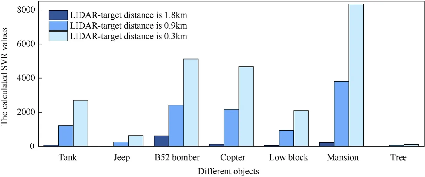
Fig. 3. SVR values of six objects in three LIDAR-object distances.
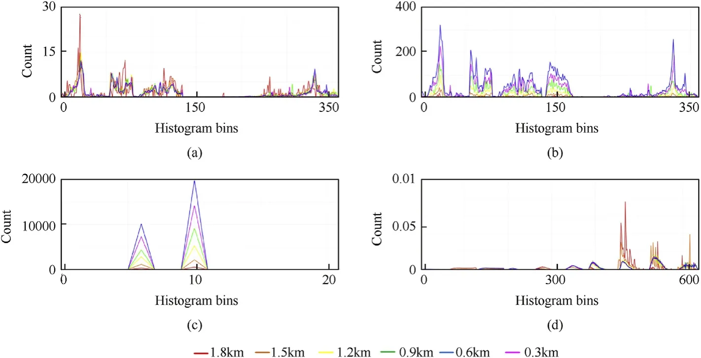
Fig. 4. Descriptor histograms of M1 Abrams model at different LIDAR-target distance under the same sensor angle as the pitch 0°yaw 0°.(a) VFH, (b) CVFH, (c)GRSD and (d) ESF.
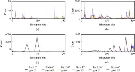
Fig. 5. Descriptor histograms of M1 Abrams model under different LIDAR angles at the 600 m LIDAR-target range. (a) VFH, (b) CVFH, (c) GRSD and (d) ESF.
Fig.6 shows that the overall recognition rate is relatively low at the maximum distance. The reason is that the number of points obtained is small at a long distance and the structural information available for identification is also relatively scarce. With the decrease of distance,the LIDAR range resolution improves,and the scene data points obtained increase accordingly. Therefore,descriptiveness of four global descriptors used is also gradually improved. Besides, ESF and CVFH have stronger descriptiveness generally than VFH and GRSD in the process of range changes.ESF contains the most information of angle, distance and area, so ESF performs best.

Fig. 6. Target Recognition performance based on the six different LIDAR-target ranges under multi angles without the SVR selection in (a) Scene1 (b) Scene 2 (c) Scene 3.

Table 3 The average recognition rate comparison between the structure without and with SVR selection.
3.1.2. Recognition experiment with SVR selection
When the aircraft is far away from the target, the relationship between points patched by LIDAR for objects of the same category is very close, and it is difficult to distinguish between targets by a single feature descriptor.But difference exists between their SVRs.Therefore, the SVR of each cluster is first compared with the interested target.
Table 3 shows that adding SVR selection brings about an average 3.325%increase in recognition rate of each descriptor(see Table 2).Among four descriptors,ESF performs best both with and without SVR selection,mainly because that ESF contains angle,distance and area information.
3.1.3. Recognition experiments with noise
We investigate the robustness of each descriptor to the Gaussian noise levels suggested by the computer vision community.Compared to Refs. [8-10,18] that apply Gaussian noise with zero mean and σ up to 0.5 Res, we study the impact of different noise intensities on target recognition with the SVR module, Gaussian noise with σ=10 cm,20 cm,30 cm was added to three scenes in the simulation process. Fig. 7 shows an example of the influence on Scene 2 with σ=10 cm, 20 cm, 30 cm Gaussian noise.
In this part, recognition experiments of simulated scenes with Gaussian noise using four descriptors are carried out and the results are shown in Fig. 8.
Fig.8 shows that the recognition of B52 bomber in Scene 2 is less affected by noise and still maintains a high accuracy rate,followed by Scene 1 which takes M1 Abrams as the target,and noise has the highest impact on jeep in Scene 3.It also indicates that ESF has the best anti-noise property, followed by VFH and GRSD, and CVFH performs the worst.
3.2. Execution time
The execution time of the whole algorithm is one of the practical factors that should be considered. This part presents the running time of the four descriptors at different ranges and each step in the whole pipeline.Scene1 was taken as the test scene,and M1Abrams as the target. Trials are implemented using Point Cloud Library(PCL) [20] in VS2017 on Windows 10 on an AMD QL-64 CPU with 4 GB RAM.
Fig. 9 shows that VFH is the fastest and ESF needs longest execution time.It indicates that ESF will be unfit for real-time use.To present an appealing ATR performance,the focus will be shifted to the CVFH and ESF.The difference of feature descriptors will only have influence on the steps “Feature extraction” and “Feature matching”.
The running time of the overall algorithm with and without the SVR selection are shown in Table 4, adding the step of SVR threshold selection decreases the execution time of feature extraction and matching and lowers the whole execution by 55.9 ms and 176 ms respectively. Especially for the ESF descriptor,adding the SVR module can reduce the total execution time by nearly the half of the original execution time.
4. Conclusion
In this paper, we propose an ATR pipeline based on global descriptors for airborne LIDAR,which contains an offline phase and an online phase. Considering point cloud data obtained by LIDAR change when the aircraft platform is at various altitudes and heights, we compare four global descriptors in three scenes. ESF performs best, then CVFH and VFH, and the last one is GRSD. Besides,results indicate that SVR can affect ATR results.What’s more,considering the real-time disturbance,ESF descriptor performs best in experiments with different levels of noise are set to compare the descriptors’robustness to noise.We propose the SVR selection and carry out corresponding experiments which win above 2.4%increment of recognition rate. And the execution time is greatly decreased, especially for the ESF descriptor.

Fig. 7. Example of Scene 2 at 300 m LIDAR -target distance with Gaussian noise of (a) σ=10 cm, (b) σ=20 cm and (c) σ=30 cm.
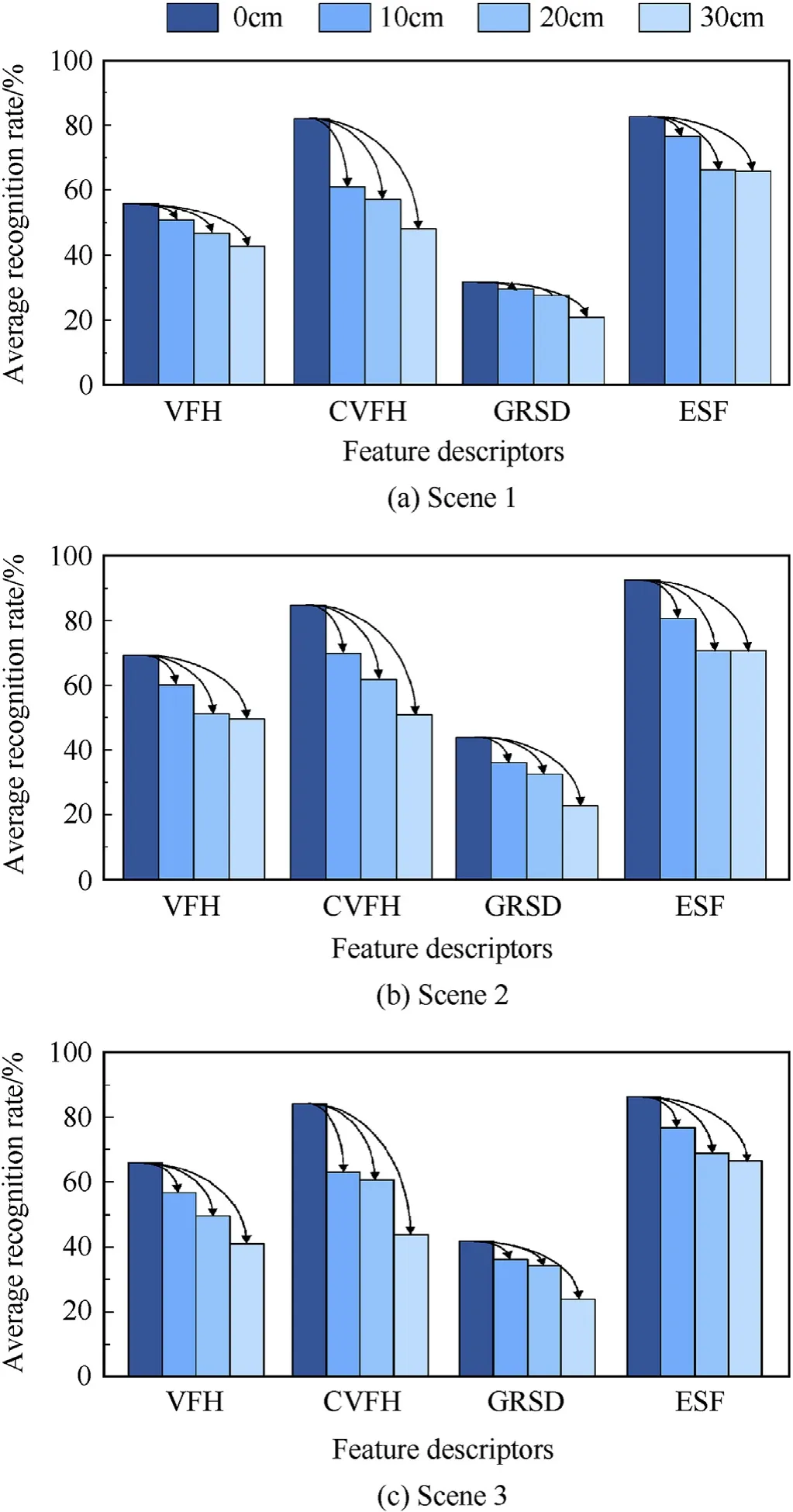
Fig. 8. Experiment results of (a) Scene 1, (b) Scene 2 and (c) Scene 3 with different degrees of noise.
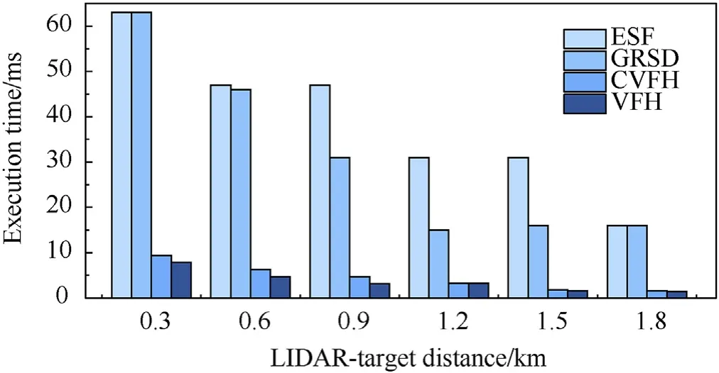
Fig.9. Execution time of four descriptors using M1 Abram model at 6 different LIDARtarget ranges.
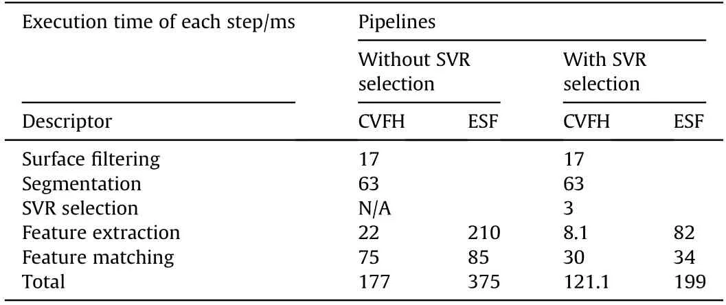
Table 4 Comparison of each step execution time using Scene 1 data at the 0.9 km range between the pipeline without SVR selection and with SVR selection.
Declaration of competing interest
There is no conflict of interest regarding the publication of this manuscript.
Acknowledgements
This research was supported by National Natural Science Foundation of China (No. 61271353, 61871389), Major Funding Projects of National University of Defense Technology (No. ZK18-01-02), and Foundation of State Key Laboratory of Pulsed Power Laser Technology (No. SKL2018ZR09).
杂志排行
Defence Technology的其它文章
- Statistical variability and fragility assessment of ballistic perforation of steel plates for 7.62 mm AP ammunition
- Texture evaluation in AZ31/AZ31 multilayer and AZ31/AA5068 laminar composite during accumulative roll bonding
- Local blast wave interaction with tire structure
- Research and development of training pistols for laser shooting simulation system
- A novel noise reduction technique for underwater acoustic signals based on complete ensemble empirical mode decomposition with adaptive noise, minimum mean square variance criterion and least mean square adaptive filter
- Research on extraction and reproduction of deformation camouflage spot based on generative adversarial network model
