Forecasting method of induced passenger flow for Sichuan-Tibet railway based on improved MD model
2020-05-10ZhangJinXuJunxiangGuoJingni
Zhang Jin Xu Junxiang Guo Jingni
(School of Transportation and Logistics, Southwest Jiaotong University, Chengdu 611756, China)
Abstract:Aiming at the limitation of forecasting induced passenger flow with the modal demand(MD) model, which assumes that the travel time value and travel utility obey the fixed probability distribution, a forecasting method of induced passenger flow is proposed by using an improved MD model based on the prospect theory. Combined with the actual traffic flow survey data of the Sichuan Tibet passenger transport channel, the improved MD model is used to forecast the total passenger flow and induced passenger flow along the Sichuan Tibet railway. Finally, the improved forecasting model is compared with the traditional MD model and the Logit model, and the effects of the parameters in the foreground theory on the forecasting results are analyzed. The results show that the Logit model forecasting result is 8.5% higher than the improved MD model forecasting result, the traditional MD model forecasting result is 3.7% higher than the improved MD model forecasting result, but the difference between the forecasting results of each model is within 10%.The parameter value in the prospect theory has a significant effect on the passenger flow forecasting results, especially in the two types of travelers, the variable and the conservative, where the forecasted difference reaches 23%.
Key words:induced passenger flow; passenger flow forecasting; prospect theory; modal demand (MD) model
In recent years, an increasing number of experts and scholars have paid attention to the research of induced passenger flow forecasting. Forecasting of induced passenger flow for new-built passenger dedicated lines can be constructed based on the RBF neural network model for short-term traffic flow forecasting according to the characteristics of high forecasting accuracy of the RBF neural network in complex network systems[1]. By analyzing the mechanism of induced passenger flow, a passenger flow forecasting model based on the TOD model is proposed, and a growth curve forecasting model based on the TOD model is established. This model mainly forecasts induced passenger flow through land use change[2], but this method is not suitable for forecasting the induced passenger flow in the initial stage of new-built high-speed railways due to the explosive manifestation of potential demand. According to the autoregressive moving average model and utility theory, the diversion passenger flow and induced passenger flow can be distinguished from each other[3]. Some scholars have quantitatively analyzed the spatial and temporal distribution characteristics of induced passenger flow, and proposed a method of using the fractal dimension theory to describe the complex characteristics and variation characteristics of induced passenger flow in urban rail transit. This method is based on the variation and distribution of passenger flow data to depict the characteristics of induced passenger flow, without considering the influencing factors of passenger travel behavior, so that it can be applied to the intersection. The research of traffic flow distribution is not suitable for the forecasting of induced passenger flow[4-5], and the limitation of this method is that the forecasting model can be applied to Beijing, Shanghai and other economically developed areas as well as areas with an obvious polarization effect in the growth pole theory. If it is a poor area, this model is no longer applicable. There are also many methods for forecasting induced passenger flows, for example using the trip distribution-mode choice (TDMC) model to forecast the increased passenger flow by public transport[6].Aiming at the train delay condition, the neural network model is used to forecast the passenger flow[7-8]. The traditional forecast method of induced passenger flow adopts the four-stage method[9-13].
The MD forecasting model is a new passenger flow forecasting method developed by the Japan Transport Administration in the 1970s. It was first applied to the passenger flow forecasting of the Shinkansen Line. Its principle is to adopt the utility theory of economics and take the individual traveling as the object to analyze the potential passenger demand, so it is very suitable for the induced increase of new-built railway lines[14-17]. The prospect theory can describe people’s risk attitudes in the face of gains or losses and explain the impact of travel utility considering travelers’ psychological expectations on passenger flow forecasting results. Therefore, this paper considers using the improved MD model based on the prospect theory to forecast the induced passenger flow after the completion of the Sichuan-Tibet railway. The main innovations are as follows:
1) The travel time value and travel utility in the traditional MD model are recharacterized by the prospect theory value function and weight function, and the travel psychological behavior of travelers is taken into consideration in the study.
2) The improved MD model is used to forecast the induced passenger flow after the completion of the Sichuan Tibet railway, and it is compared with the traditional forecasting model to verify the rationality of this method.
3) This research shows the influence of different parameters in the value function and weight function of the prospect theory on the forecasting results, and analyzes the influence of travelers’ different travel psychological preferences for the forecasting results.
1 Theory and Method
The prospect theory was proposed by Kahneman and Tversky in 1979[18]. It is a descriptive theory, which assumes that the decision maker is limited in rationality, that the individual’s ability to calculate and think is limited, and that the judgment information of the options is not fully determined. The prospect theory holds that the decision maker will receive the first satisfactory result compared with the expected reference point, but not necessarily the result of the greatest benefit[19].In the prospect theory, value functionv(x) and decision weight functionw(p) are usually used to describe individual decision-making behavior.The value function is a subjective function, which represents the difference between the current value and the reference point, in which the reference point is determined by the subjective judgment of the decision maker. The decision weight function is a subjective probability function, which is the subjective judgment made by the decision maker according to the probability in the expected utility theory.The value function and the decision weight function together constitute the prospect function, which affects the final decision of the decision maker. The specific form of the prospect function is
Vi=w+(p)v+(x)+w-(p)v-(x)
(1)
whereVirepresents the comprehensive prospect value;v+(x) represents the profit value function;w+(p) represents the profit weight function;v-(x) represents the loss value function;w-(p) represents the loss weight function.
Profit value function(v+(x)) and loss value function (v-(x)) are expressed as
(2)
where Δxrepresents the difference between the actual decision result and the reference point;σrepresents the profit pursuit coefficient;λrepresents the loss avoidance factor. In the actual decision-making process, there is a natural endowment effect. When people own an item, their evaluation value of the item is much higher than before. Therefore, when people lose the item, they expect to sell it at a high price. Therefore, the acquiescence of profit pursuitσis 1, so the value function can be expressed as
(3)
Whenλ>1, it means that decision makers are more sensitive to losses than to gains.αrepresents a diminishing marginal sensitivity parameter for revenue, andβrepresents a marginally sensitive decreasing parameter for loss, 0<α<1, 0<β<1.
The prospect theory holds that people tend to overestimate probability events and underestimate probability events in decision-making, but they are relatively insensitive to the change of intermediate probability. The expression of decision weight function is
(4)
whereωis the risk-return attitude coefficient;μis the attitudinal coefficient of risk loss.
At present,the prospect theory has been widely applied in many fields, such as route selection[20], mode selection[21], dynamic traffic flow allocation[22], and emergency plan decision-making[23], and many valuable research results have been obtained.
Several basic concepts in the MD model include the potential passenger demand, travel utility, travel sacrifice, time value and potential demand manifestation rate, which can describe the mechanism of induced passenger flow as described above[24].Therefore, it is suitable to use the MD model to research the induced passenger flow forecast caused by the explosive growth of demand in the near future after the completion of high-speed rail lines[25].The variation of the induced passenger flow is shown in Fig.1.

Fig.1 The variation of induced passenger flow
The interpretations of the potential passenger demand, travel utility, travel sacrifice, time value and potential demand manifestation rate in the MD model are as follows:
1) Potential passenger demand.In the MD model, the potential passenger demand is defined as the total number of potential passengers who may displace from the origin to the destination. In the MD model, potential passenger demand refers to the number of people who do not consider the ability to pay between OD as long as they have the intention to travel.
2) Travel utility.Travel utility in the MD model refers to the value or benefit that travelers gain through this trip, such as travel, trade, school, etc.The MD model holds that people are willing to travel because they want to obtain travel utility. The level of social and economic development of the region determines the general level of travel utility. The travel utility is also related to the characteristics of travelers. The traditional MD model assumes that the evaluations of travel utility obeys the lognormal distribution, and all OD pairs present this kind of distribution.However, it should be noted that the travel utility in the MD model is different from that in the traditional four-stage forecasting model. The value of travel utility in the MD model is only related to the traveler’s own factors. It is a subjective psychological evaluations of whether the traveler can satisfy his/her inner desire to travel. Price has no direct impact on the specific mode of transportation and its service characteristics, while the travel utility in the traditional four-stage forecasting model is related to both[26].
3) Travel sacrifice. In the MD model, the traveler’s cost to obtain the travel value is called the travel sacrifice. This cost is a generalized cost including travel time consumption, travel cost, travel fatigue, etc.
4) Time value.Time value refers to the monetary manifestation of the added value of benefits and the loss of benefits caused by the consumption of time. Different travelers have different evaluations of time value, which is due to the different evaluations of time value by different travelers for different purposes and time-consumption[27]. In the MD model, it is also assumed that the evaluation of time value also obeys lognormal distribution.
5) Potential demand manifestation rate.When the traveler’s travel utility is greater than the traveling sacrifice of the mode, that is to say, the benefit is more than the cost, the potential transport demand will be realized, which is called the manifestation of the potential transport demand. This part of passenger flow formed after the manifestation of the potential demand is called the passenger demand volume, and its proportion in the total potential passenger demand volume is called the latent demand manifestation rate.
2 Forecasting Process of Induced Passenger Flow
2.1 Determination of time value
In the specific transportation process, if travel time is not consumed in this way, then it can be used for other labor productions and create economic benefits and value. Therefore, the authors assume that the economic value created in unit time is equivalent to the time value of travelers. The expression of the decrease in income caused by the time consumed in travel which leads to the incapacity to work is
(5)
(6)
2.2 Determination of travel sacrifice quantity
1) Travel time consumingT. Travel time is the total time spent by the chosen means of transport in the whole OD, including the travel time during the journey and the connection time between the start and end of the journey and the station. As the research object of this paper is the newly built railway, without considering other modes of transport, it can be expressed as
(7)

f(T)=viT
(8)
2) Travel expensesC. Travel expenses are the total expenses that travelers spend in the process of traveling. They can be expressed as
(9)
whereCirepresents the total cost in the travel process. Assuming thatf(Ci) represents the contribution value of passenger travel expenses to travel sacrifices, the monetary unit dimension can be expressed as
(10)
3) Travel comfortG(t). Different modes of transportation will bring different feelings of comfort to passengers. There are many factors affecting the comfort degree of passengers, such as stability, seat comfort, the internal environment, service quality, etc. The authors consider using the travel fatigue recovery time of travelers to quantify the comfort degree, which can be expressed as
(11)
whereRmaxrepresents the longest time it takes to recover from travel fatigue;γis a dimensionless parameter, representing the minimum travel fatigue recovery time;τrepresents the fatigue recovery time intensity factor per unit travel time. According to Ref.[28], whenRmax=15, the value of parameterτis 0.28. Assume thatf(G) represents the contribution value of the comfort degree to travel sacrifice, which is the same as that of travel time quantification. The comfort degree is converted into a monetary unit dimension by unit time value, which can be expressed as
f(G)=viG(t)
(12)
4) Travel safety.Travelers need to bear the risk of travel when choosing the mode of transportation. The authors quantify the safety of travel by using the rate of travel accidents. The rate of travel accidents is defined as the number of passenger casualties that occur within 1.0×10⁸km of passenger turnover in a certain period of time. The following expression can be used to express the number of passenger casualties that occur within 1.0×10⁸km of passenger turnover.
(13)
whereεrepresents the accident rate;Arepresents the passenger traffic volume;Lrepresents mileage. Assume thatf(ε) represents the contribution value of safety loss to travel sacrifice. The amount of compensation after the accident is converted into a monetary unit dimension, which can be expressed as
f(ε)=θε
(14)
According to the national policy in China, the limit of liability for personal injury and death of railway passengers caused by accidents is 150 000 yuan, so the value is 150 000 yuan.
In the MD model, the amount of travel sacrifice is affected by travel time, travel cost, travel comfort and travel safety. The formula for calculating the amount of travel sacrifice can be obtained by adding the contribution values:
(15)
2.3 Determination of travel utility
The traditional MD model considers that the travel utility of travelers is the same as the time value and obeys lognormal distribution. It has been analyzed above that the travel utility of the MD model is only related to the traveler himself, and different travelers have different travel utilities. Therefore, the traveler’s travel benefit can be described by the value function and decision weight function in the prospect theory. The authors believe that the traveler’s expectation of travel benefit can be reflected by the comprehensive prospect value function of travel, which can be expressed as
(16)
(17)

(18)
f(Vi)=(f(lnu))αw+(f(lnu))+
(f(lnu))βw-(f(lnu))
(19)
Travel utility can be described by Eqs.(16) to (19). Eq. (16) represents the expression of travel utility in the traditional MD model. Assume thatηlnuis the logarithmic mean of travel utility andφlnuis the logarithmic variance of travel utility.μandσare the traditional mean variance symbols, which are used in Eqs.(2) and (4), so the symbols are replaced here.Eq.(17) denotes the value function in the prospect theory, Eq.(18) denotes the decision weight function in the prospect theory, and Eq.(19) denotes the comprehensive prospect function, which is used here to denote travel utility.
2.4 Determination of potential demand and potential demand explicit rate
According to the forecasting principle of the MD model, the combination formula can be expressed as
(20)
whereRn,ijrepresents the potential passenger manifestation rate for selecting modenfrom nodeitoj;qn,ijdenotes the passenger volume from nodeitojto choose the mode of transportn;Qijrepresents the potential passenger traffic volume of modenchosen fromitoj;vn+1,nandvn,n-1represent the border substitution rates between modes of transportation. Potential passenger demand can be expressed as follows and potential passenger demand changes are shown in Fig.2.
(21)
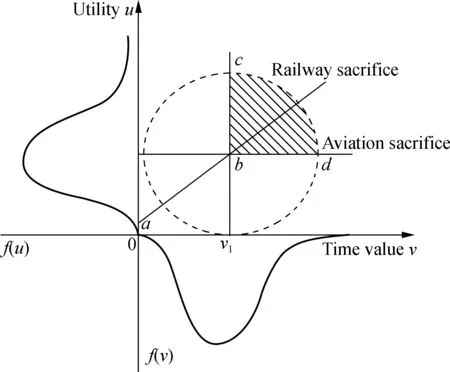
Fig.2 Potential passenger demand change chart
The forecast steps of the induced passenger flow based on the improved MD model are shown in Fig.3.

Fig.3 Flow chart of induced passenger flow forecasting
3 Forecasting of Induced Passenger Flow
3.1 Introduction for the Sichuan-Tibet Railway
Located in Sichuan Province and the Tibet Autonomous Region of China, the Sichuan-Tibet railway, with a total length of 1 838 km, is a fast railway connecting Sichuan Province and Tibet Autonomous Region. It is the second railway to enter the Tibet in China and one of the trunk railways in southwest China[29]. The traffic zones along the Yalin section of Sichuan-Tibet Railway can be divided into the Ganzi Tibetan Autonomous Prefecture, Changdu area, Linzhi area and Shannan area.
3.2 Current situation of traffic passenger volume
3.2.1 Highway passenger flow
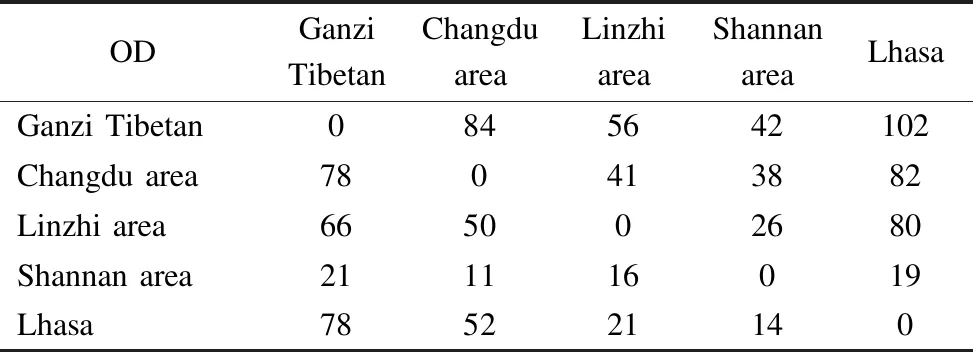
The Highway along the Sichuan-Tibet Railway is dominated by the G317 and G318 national highways. Combining the traffic investigations in G317 and G318 and collating the OD survey data of motor vehicles in relevant station statistical reports, the passenger flow tables of highway passage sections along the Sichuan-Tibet Railway in 2018 (base year) are shown in Tab.1.
Tab.1 OD table for highway passengers in alpine areas along the Sichuan-Tibet railway in the base year 104person/a
ODGanzi TibetanChangdu areaLinzhi areaShannan areaLhasaGanzi Tibetan0845642102Changdu area780413882Linzhi area665002680Shannan area211116019Lhasa785221140
3.2.2 Air passenger flow
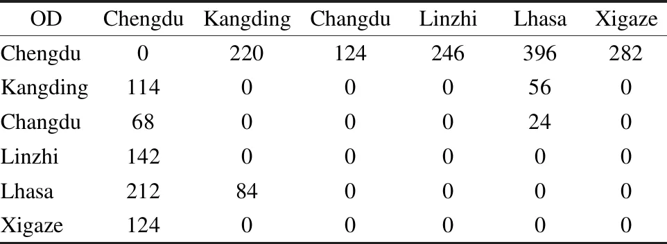
Since there are almost no direct flights on the air airport routes along the Sichuan-Tibet Railway in alpine areas, the Kangding-Lhasa flights on the only route are very few, and the annual passenger flow is very low. It is not useful to count the air traffic in the alpine areas along the Sichuan-Tibet Railway. Therefore, the research considers that for the main statistics of air transport corridors, the passenger flow of the whole line of the Chuan-Tibet Railway has practical significance for the future research of the passenger flow transfer caused by the new construction of the Sichuan-Tibet Railway.The specific air passenger flow statistics are shown in Tab.2(The statistical passenger flow is direct passenger flow). The actual total air passenger flow of the Sichuan-Tibet Railway in the frigid areas studied in this paper only includes Kangding, Changdu, Linzhi and Lhasa.
Tab.2 Air OD table of Sichuan-Tibet area in the base year 104person/a
ODChengduKangdingChangduLinzhiLhasaXigazeChengdu0220124246396282Kangding114000560Changdu68000240Linzhi14200000Lhasa212840000Xigaze12400000
3.2.3 Passenger flow in corridor
Combining the passenger flow density of the above two modes of transportation, the passenger flow in the attraction range of the transportation modes in the Sichuan-Tibet area in 2018 is shown in Tab.3.
Tab.3 Passenger flow and market share of two transportation modes in Sichuan-Tibet region

TransportationPassenger flow/(104 person·a-1)Market share/%Highway transport97758.3Trans70041.7Total1 677100
3.3 Improvement of MD model forecasting based on the prospect theory
According to the data of the current investigation, the passenger volume operation of the Sichuan-Tibet Railway in the alpine regions after its completion is studied and forecast. The forecast base year is 2018, and the total OD of the current passenger flow is 16.77 million. Since the Sichuan-Tibet Railway is expected to open to traffic in 2030, the forecast year is set to be 2035 in the near future and 2040 in the mid-term.
The calculation steps of the improved MD model based on the prospect theory are as follows:
1) Calculation of time value
After completing the preparatory work of the data collection, questionnaire survey and traffic district division, the expected reference points of time value for people in this area are determined by Eq.(5) according to the regional economy and population, and the values ofλandβin Eq.(6) are obtained by a questionnaire analysis, so as to obtain the the information of travelers in this area. This paper includes a questionnaire designed to help understand the travel characteristics of people in Sichuan and Tibet. Through data analysis, we obtain the values of parametersλandβof the prospect theory in Eq.(5), which are 1.38 and 0.59, respectively.
2) Calculation of traffic sacrifice
The travel time and fare of transportation corridors in Sichuan and Tibet were collected, and the travel comfort of people was investigated by designing questionnaires for different travel modes. The contribution values of different factors affecting travel sacrifice are calculated by combining Eqs.(7) to (14). Eq.(15) is used to sum the contribution values of each influencing factor, and the base and target annual values of the line sacrifice are calculated.
3) Calculation of traffic utility
Through the analysis of the questionnaire and the calculation results of passenger flow and time value of different modes of transportation between OD pairs, the values of parametersα,β,ω,μandλbased on the foreground theory model are obtained. The travel utility can be obtained by substituting Eq.(16) into Eq.(19). In this paper, the values of theoretical parameters of foreground in Eq.(16) and Eq.(19) are obtained by data analysis through questionnaires,α=0.34,β=0.46,ω=1.12,μ=0.82,λ=1.58.
4) Calculation of the potential demand manifestation rate
According to the calculation of the apparent rate of potential demand, the relevant parameters obtained above are substituted into Eq.(20), and the upper and lower bounds of the integral are substituted for the substitution rate of the boundaries of different modes of transportation. Then the basic annual valueR0n,ijand the target annual valueRtn,ijof the apparent rate of different OD pairs of transportation modes can be obtained.
5) Estimation of potential passenger demand in the base year
By dividing the passenger demand between base year intervaliandjby the apparent rate of potential demand in the base year, the potential passenger demand in the base year, i.e. Eq. (21) is obtained.
6) Calculation of potential passenger transport demand in the future year
Based on the socio-economic and demographic data of the base year of a traffic district, the potential passenger demand of the base year calculated in the previous step is used to determine the potential passenger demand function of the target year. Then, the forecasting value of the socio-economic population index of the target year is substituted into the potential passenger transport demand function, and the potential passenger transport demand of the target year is obtained.
7) Calculation of passenger transport demand in the coming year
Passenger demand in the coming year is calculated according to the potential demand dominance rateRtn,ijand obtained potential passenger demandQt,ij.
qtn,ij=Qt,ijRtn,ij
(22)
8) Transfer of passenger traffic
The transfer of passenger traffic is due to the change of traffic mode between OD and OD after the opening of the railway line. This part of passenger flow is divided into a new railway, that is, the transfer of passenger traffic. The calculation formula is
M=Qt-Q0
(23)
whereMdenotes the transfer of passengers after the construction of a new railway;Qtindicates the passenger flow of existing modes of transport when there are no new modes of transport in the coming year;Q0indicates the passenger flow of existing modes of transport when new modes of transport are added in the coming year.
9) Induced passenger flow
The induced passenger flow of the newly built railway can be expressed by the following formula according to the description above:
Qt,ij=qt,ij-Mt,ij
(24)
whereQt,ijdenotes the induced passenger flow of the newly built railways in intervalsitojin the coming year;qt,ijrepresents passenger flow betweeniandjin the next year;Mt,ijrepresents the sum of passenger flow transfers from existing modes of transport in the coming year.
From the forecasting steps above, we can obtain the forecast of passenger flow in the alpine area along the Yalin section of Sichuan-Tibet Railway in the future. The results are shown in Tab.4.
Tab.4 Forecast results of passenger flow along Sichuan-Tibet Railway in the alpine region 104person/a

Forecast year20352040Sichuan-Tibet Highway9471 120Transport Aviation8621 094Sichuan-Tibet Railway1 5802 350
From this, we can obtain the forecast results of the induced passenger flow in the alpine areas along the Sichuan-Tibet Railway as shown in Tab.5.
Tab.5 Forecast results of induced passenger flow in the alpine areas along the Sichuan-Tibet Railway 104person/a

Forecast year20352040Induced passenger flow 1 7122 887
3.4 Comparative analysis of forecasting model
In order to verify the accuracy and reliability of the MD model for the forecasting results of induced passenger flow of the newly-built Sichuan-Tibet Railway, this paper uses the improved MD model based on the prospect theory, the Logit model in the four-step forecasting method, and the traditional MD model to compare the forecasting of total induced passenger flow in 2035 in the areas along the line. The results are shown in Fig.4.
It can be seen from Fig.4 that the results of the improved MD model are lower than those of the traditional MD model and Logit model. For induced passenger flow forecasting, the Logit model forecasting results are 8.5% higher than the results in this paper, and the traditional MD model forecasting results are 3.7% higher than the results in this paper, but the difference between the forecasting results of each method is within 10%. This shows that the forecasting method based on the improved MD model proposed in this paper shows reliability in the research of induced passenger flow forecasting.
3.5 Analysis of the influence of parameters α and β on the results
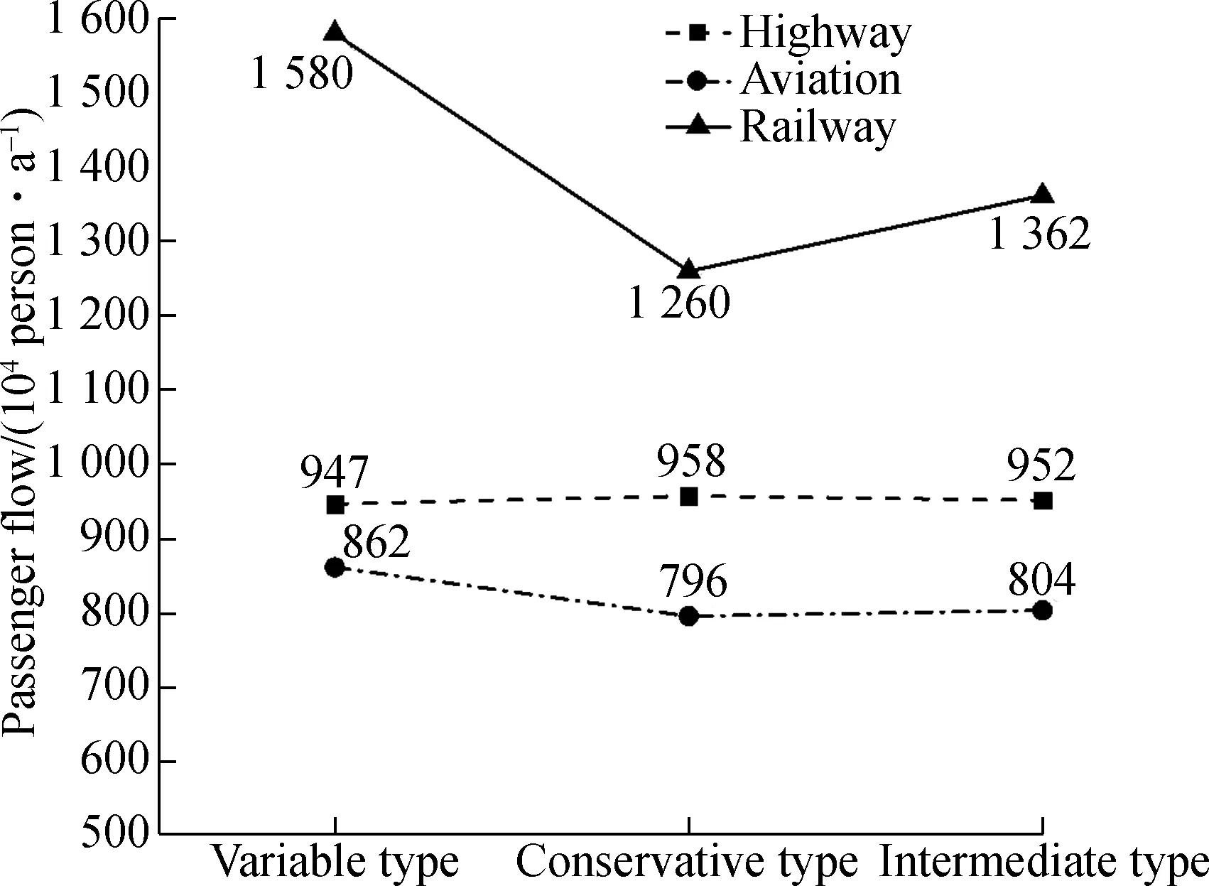
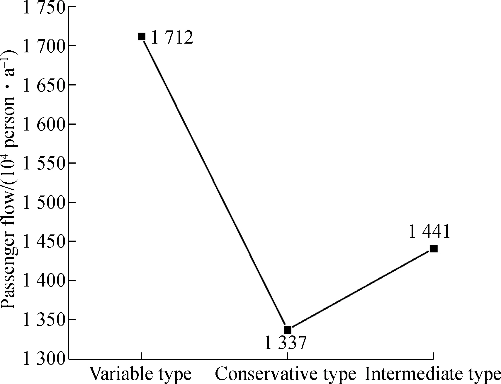
The values of parametersαandβin the value function of the prospect theory reflect the travelers’ psychological behavior of travel decision-making. This paper discusses the effect of parameters on the forecasting results by comparing the fluctuation of passenger flow in different modes of transportation and the changes of induced total passenger flows under different values. The specific parameter values are shown in Tab.6, and the impact of the forecasting results is shown in Fig.5.

(a)

(b)
From Fig.5, it can be seen that the effect of different parameters and values on the forecasting results is quite different, especially for the two types of traveler pairs, which are variable and conservative. Therefore, it can be seen that the improved MD model based on the prospect theory is important for the analysis of the effect of parameter values on the forecasting results in the prospect theory. Using this method, we need to fully investigate the
Tab.6 Parameter value characteristics of travelers between traffic OD and accurately describe the parameter value of the prospect theory.

Traveler categoryParameter value rangeParameter valueVariable type0<α,β<1α=0.34,β=0.46Conservative typeα>1,β>1α=2.25,β=1.62Intermediate typeα=β=1α=β=1
(a)
(b)
4 Conclusions
1) Based on the prospect theory, it is feasible and applicable to improve the forecasting method of the MD model to forecast the traffic flow of the railway under construction.
2) The forecasting model based on the prospect theory describes travelers’ psychological behavior, so the forecasting result will be more accurate than those of the traditional methods.
3) The parameter value in the prospect theory reflects travelers’ travel decision preference, which has a great impact on the passenger flow forecasting results. Therefore, it is necessary to accurately depict the characteristics of regional travelers in the future research.
杂志排行
Journal of Southeast University(English Edition)的其它文章
- The walking distance decay law of amenity selection based on binary logistic model
- Evaluation of rutting and low-temperature cracking resistancesof warm-mix recycled asphalt bindersunder the secondary aging condition
- Effects of curing age on compressive and tensile stress-strain behaviors of ecological high ductility cementitious composites
- Dispersion of graphene in silane coupling agent aqueous solutions
- An explicit representation and computation for the outer inverse
- The cause of human fatigue and scenario analysisin the process of marine transportation
