Computational fluid dynamics simulation of Hyperloop pod predicting laminar-turbulent transition

Nathalie Nick·Yohei Sato

Abstract Three-dimensional compressible flow simulations were conducted to develop a Hyperloop pod.The novelty is the usage of Gamma transition model,in which the transition from laminar to turbulent flow can be predicted.First,a mesh dependency study was undertaken,showing second-order convergence with respect to the mesh refinement.Second,an aerodynamic analysis for two designs, short and optimized, was conducted with the traveling speed 125 m/s at the system pressure 0.15 bar.The concept of the short model was to delay the transition to decrease the frictional drag;meanwhile that of the optimized design was to minimize the pressure drag by decreasing the frontal area and introduce the transition more toward the front of the pod.The computed results show that the transition of the short model occurred more on the rear side due to the pod shape,which resulted in 8%smaller frictional drag coefficient than that for the optimized model.The pressure drag for the optimized design was 24%smaller than that for the short design,half of which is due to the decrease in the frontal area,and the other half is due to the smoothed rear-end shape.The total drag for the optimized model was 14%smaller than that for the short model. Finally, the influence of the system pressure was investigated.As the system pressure and the Reynolds number increase,the frictional drag coefficient increases,and the transition point moves toward the front,which are the typical phenomena observed in the transition regime.

Keywords Computational fluid dynamics(CFD)·Drag·Subsonic compressible flow·Hyperloop·Laminarturbulent transition

1 Introduction

In Switzerland,a national project called Swissmetro was conducted in which a high-speed magnetic levitation(maglev)passenger train system running in an underground vacuum tunnel was supposed to be developed.The concept of Swissmetro was originally proposed by Nieth[1]during the 1970s,a schematic of which is shown in Fig.1a.Unlike other maglev projects,e.g.,the German Transrapid,Japanese JR-Maglev MLX, and Inductrack in the USA,Swissmetro employed the concept of a vacuum tunnel for the purpose of a drag reduction of the train.Preliminary and feasibility studies were undertaken at the Swiss Federal Institute of Technology Lausanne(EPFL),and the project was conducted by EPFL and the company Swissmetro AG from 1994 to 1998,with sponsorship given by the Swiss National Science Foundation[2].The Swissmetro system features numerous advantages,including a low energy consumption,high speed,low noise,and immunity to weather such as snow and storms.However,mainly owing to the necessity of an immense initial investment for building an underground vacuum tunnel,the project was stopped, and Swissmetro AG was liquidated in 2009.However,after a decade,this transport system has been refocused for development in Switzerland.The next generation of the Swissmetro AG project(SwissMetro-NG)(https://swissmetro-ng.org/)has been recently promoted by the Swiss parliament as a next-generation transportation system for Switzerland as a way to cope with technologies required for a new transport system.Another vacuum transportation project is in process in Switzerland.The EuroTube Foundation (https://eurotube.org/) aims to accelerate the breakthroughs in vacuum transportation and to build a 3-km-long vacuum tube to offer European universities and companies a research center in Collombey-Muraz, Canton of Valais, Switzerland. The canton of Valais, the municipality of Collombey-Muraz and the Swiss Federal Railways have already committed themselves by actively supporting the project.

In USA,Oster proposed an Evacuated Tube Transport(ETT)system in 1997[3].The basic concept of ETT system resembles to Swissmetro,i.e.,capsules carrying passengers or cargo travel on frictionless maglev system in evacuated tubes.The passenger compartment of ETT is shown in Fig.1b.Oster envisaged a worldwide transport system including intercontinental routes,and the designed operation speed is 600 km/h for local trips and 6,500 km/h for international travel[4].As a prototype of the ETT system,the world’s first high-temperature superconducting maglev evacuated tube transport(HTS Maglev-ETT)test system was built in Southwest Jiaotong University in 2014[5].

Musk published the Hyperloop Alpha concept for use in the USA[6],the basic idea of which is similar to ETT in that pressurized capsules,or the so-called pods,travel in reduced-pressure tubes.The thrust force was provided by linear induction motors and axial compressors,which differs from ETT.Musk proposed his new transportation system as an alternative to the California high-speed rail(https://www.hsr.ca.gov/),connecting between San Francisco and Los Angeles.Feasibility studies of the Hyperloop concept were also undertaken by NASA with respect to the cost and technical aspects[7-9],and the organization provided a high-level evaluation of Hyperloop in terms of its commercial potential, environmental impact, costs,safety issues,and regulatory and policy issues,as well as to identify further research topics related to the technology.Four years after the Hyperloop Alpha paper was published,the first Hyperloop pod competition was held by the private company SpaceX.The Hyperloop pod competition is an engineering contest involving university students from all over the world with the goal to accelerate the development of the Hyperloop concept.The SpaceX Hyperloop test track was constructed in Los Angeles in 2016,which is a subscale model of the Hyperloop system.The track is straight with the length 1.25 km and an outer tube diameter of 1.8 m.

The Hyperloop team of the Swiss Federal Institute of Technology(ETH Zu¨rich)is called Swissloop(https://swissloop.ch)and competed in the competition in 2017,2018 and 2019.The Swissloop Hyperloop pod of 2017 had a cold-gas propulsion system based on compressed air that exits the pod at low temperatures and expands at the nozzles,providing a rocket-like acceleration.The pod traveled on wheels and was not levitated.In the competition conducted in 2018,the Swissloop pod was equipped with wheels propelled by electric motors.In the competition in 2019,the Swissloop team developed a linear induction motor(LIM)and was among the first teams ever to compete with this propulsion system.2019 was the first year that some few teams competed with a LIM.The final criterion to win the competition is the maximum speed.In this paper,we describe the aerodynamic analysis for the pod for the competition in 2019.

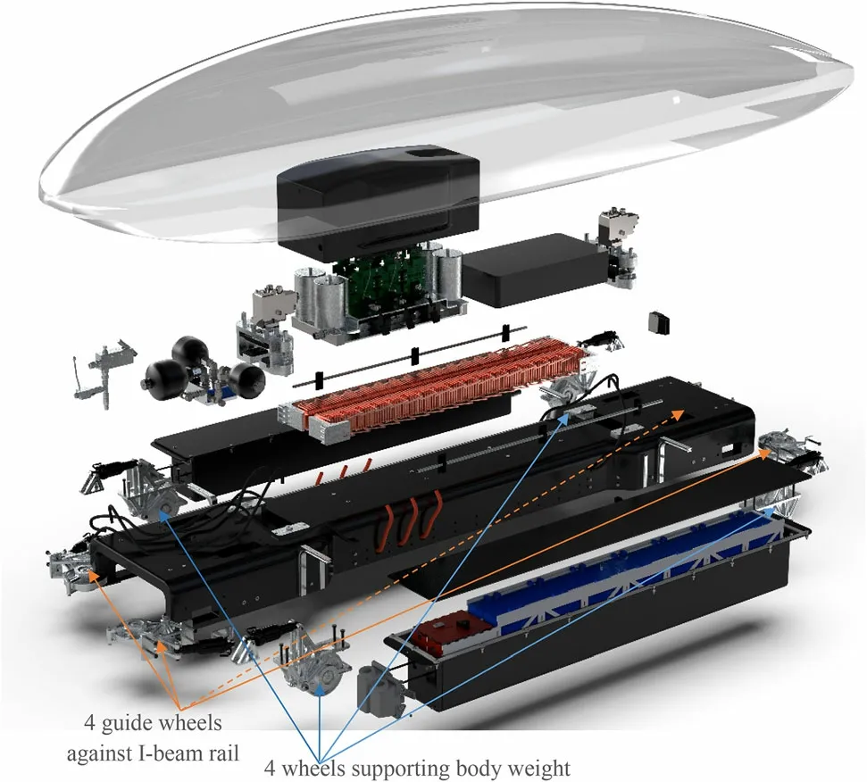
Fig.2 Swissloop’s Hyperloop pod system

The Swissloop’s Hyperloop pod is illustrated in Fig.2.A double-sided LIM is selected as the propulsion system.The body is not levitated by magnetic force,and the body weight is supported by wheels,which are not propelled.The electric power for the propulsion system is provided by batteries mounted in the pod in accordance with the rules of the competition.Because the wheels are not propelled,the adhesion between the wheels and the ground does not play an important role in terms of the acceleration of the pod.Therefore,a downforce,usually required for racing cars to increase their adhesion,is not required for our pod.The weight of the pod is approximately 200 kg,and the lift force must be lower than that to avoid taking off from the ground.The target traveling speed of the pod is subsonic at 125 m/s under 0.15 bar.Because of the limited budget and period of the project,we designed the pod shape using the results of a computational fluid dynamics(CFD)simulation,and no wind tunnel tests were conducted.

The aerodynamics of a train/pod in a partially vacuumed tube has been studied by several research groups by using CFD.Zhang presented a CFD simulation for a subsonic train in an evacuated tube[10],in which axisymmetric,incompressible flow computations were performed for a train running at a speed of 50-300 m/s under a system pressure of 10-10,000 Pa.The influence of the blockage ratio(BR)on the drag is evaluated in this study.Herein,BR is the ratio of the frontal area of a pod/train to the sectional area of a tube/tunnel.Chen et al.[11]simulated flow around maglev trains in an evacuated tube using ANSYS FLOATRAN code. Two-dimensional incompressible flow calculations were performed with different vacuum pressures,blockage ratios and design of trains.They concluded that the blockage ratio of 0.25 is efficient in terms of drag reduction at the tube pressure 1,000 Pa.A three-dimensional CFD analysis of a Hyperloop pod was first reported by Braun et al.[12],who proposed a procedural system for an aerodynamic design,in which a preliminary analysis was conducted in one dimension,followed by a three-dimensional analysis for optimization.Opgenoord and Caplan presented an optimization of the Hyperloop pod developed by the team from the Massachusetts Institute of Technology(MIT)[13].The design speed was Mach 0.3,although a transonic speed was also analyzed to evaluate the influence of the choke flow around the pod on the drag force.Oh et al.[14]used CFD for an analysis of the aerodynamic characteristics of the Hyperloop system.In their study,large parametric studies were performed for the drag of the pod with different BRs,pod lengths,speeds and tube pressures.

From the viewpoint of drag reduction,the laminar-turbulent transition is an important physical phenomenon since it has significant influence on the drag,especially when the Reynolds number,Re,is near the critical Reynolds number,Recrit.Note that Recritfor a flat plate is 5×105-106[15].In the laminar flow regime,the skin friction is low,which is desirable with respect to the drag reduction.However,once the flow separation occurs in the laminar flow regime,it tends to cause a large increase in the pressure drag owing to a massive flow separation.Meanwhile,the skin friction is larger in the turbulent flow owing to the existing vortices,although the pressure drag is lower than that in the laminar flow regime.In case of highspeed trains,the Reynolds number is of the order of 107-8,which is far beyond Recrit,and the transition does not have large impact on the drag.However,mainly because of the short length of the Hyperloop pod,the Reynolds number is of the order of 106for the subsonic case,and thus,the transition may play important role with respect to the drag.

Table 1 Principal dimensions of short and optimized models

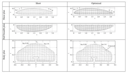
Fig.3 Comparison of pod shape between short and optimized models in m

Nonetheless, the CFD studies mentioned above[10-12,14]assumed that the whole computational domain is fully turbulent and the laminar flow and the transition were neglected.Only Opgenoord and Caplan[13]paid attention to the transition.In their two-dimensional CFD simulations,the transition was modeled with eNmethod[16],which is based on the linear stability theory[17].The simulation result for Re=6×105showed that the transition occurs closer to the nose(front)if the nose shape is blunt,which was considered to be reasonable.They also demonstrated a three-dimensional CFD simulation,but the fully turbulent flow was assumed for this case.To the authors’knowledge,no one has performed a three-dimensional CFD simulation for Hyperloop pod,taking into the laminar-turbulent transition.

In this paper,we present an analysis of the aerodynamics of a Hyperloop pod using three-dimensional CFD,taking into account the laminar-turbulent transition.All CFD simulations described in this paper were conducted in three dimensions,and the air was modeled as a compressible fluid.We focused particularly on the drag of the pod because(1)only the maximum speed was compared in the competition,and(2)the lift force was deemed unnecessary because the pod is not levitated.To predict the point of the laminar-turbulence transition,rather than prescribing it,we use a Gamma transition model[18],which is one of the original aspects of this study.The commercial CFD code STAR-CCM+Version 13 is used for the simulations.

2 Numerical method

In this section,we briefly describe the governing equations and numerical schemes used in this paper.The governing equations for a compressible flow,i.e.,the conservation of mass,momentum,and energy,are,respectively,defined as follows:

where ρ is the density,t the time,u the flow velocity vector,I the unit vector,p the pressure,τ the viscous stress tensor,E the total energy,q the heat flux vector,and ⊗denotes the Kronecker product.The total energy E can be defined using the volumetric heat capacity cpand the temperature T as

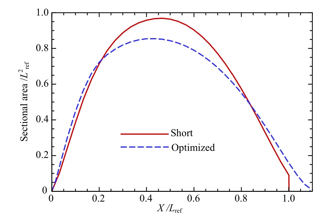
Fig.4 Comparison of sectional area curve between short and optimized models

In this paper,the air is assumed to be an ideal gaswhere R is the specific gas constant.

The finite-volume approach is used for the spatial discretization.The inviscid flux is calculated based on Roe’s flux-difference splitting scheme [19], and the viscous fluxes are discretized using a second-order-accurate centered-differencing scheme.The coupled flow solver,in which the conservation equation for the mass,momentum and energy are solved simultaneously through vector equations,is employed.A steady-state assumption is used,and the implicit Euler scheme is employed for the discretization in the pseudo-time step.

A turbulent flow is modeled using the shear-stress transport(SST)k-ω model[20]coupled with a Gamma transition model[18].This approach was selected because the Gamma transition model is able to predict the transition from laminar to turbulent flow without prescribing the location of the transition,although several coefficients are still based on the correlations.The formulation of the Gamma transition model includes one transport equation for the turbulent intermittency γ,which practically indicates the degree of the turbulent flow regime,namely,γ=1.0 for a fully turbulent flow and γ=0 for a laminar flow.The verification and validation of this laminar-turbulent transition model implemented using the STARCCM+code are reported in[21].The drawback of the Gamma transition model is a requirement of a fine mesh,namely,the mesh size must be smaller than 0.5%of the pod length. To calculate the flow field in a viscous boundary layer,the wall function is not used in this study.The overview and the details of the laminar-turbulent transition models,which can be coupled with CFD code,are reviewed in[22].

3 Conditions of simulation

3.1 Pod design

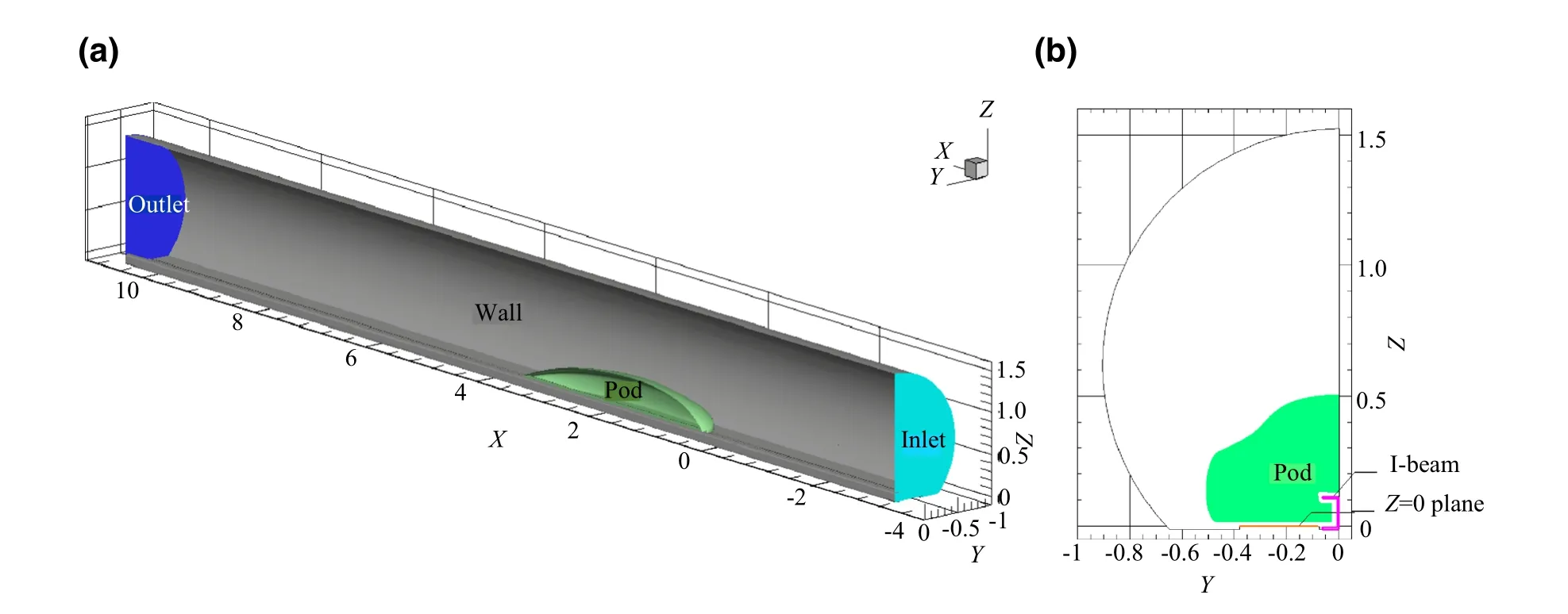
Fig.5 Computational domain:a perspective and b rear views,in m

Fig.6 Surface mesh on the pod(a)and mesh on the symmetry plane(b)

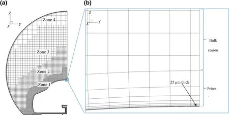
Fig.7 Computational mesh on the sliced plane at X=1.5 m:a entire and b magnified views

For the Hyperloop competition in 2019,the Swissloop team designed more than 20 outer pod shapes to achieve a drag reduction.The design variables were the pod length,width,height,frontal area and three-dimensional shape.The objective function is only the minimum drag force.Note that the thrust force of the Swissloop pod is given through the LIM instead of the driving wheels.Thus,the downforce that is typically required for racing cars to improve tire adhesion is not essential for our pod.All wheels shown in Fig.2 are omitted in the CFD simulations to simplify the geometry.Because of the limited project period,we did not optimize the pod shape using an automated optimization such as the genetic algorithm(GA)or sequential quadratic programming (SQP) [23]. The improvement in the design was undertaken by trial-anderror,incorporated with the knowledge obtained from the CFD results.

In this paper,we present two models,namely short and optimized,as the representative designs.The concept of the short model is to delay the laminar-turbulent transition and decrease the frictional drag.Meanwhile,the optimized model was designed to minimize the pressure drag by(1)decreasing the frontal area and(2)introducing the laminarturbulent transition more toward the front of the pod.To avoid a flow separation,both models were streamlined.The principal dimensions of the two models are listed in Table 1,where L,B,and H are the length,breadth,and height of the body,respectively.Apodis the frontal area of the pod,S is the surface area of the pod,and the blockage ratio,BR,is defined as follows:

where Atubeis the sectional area of Hyperloop tube.

The pod shape is shown in Fig.3.Referring to the shear plan,the maximum height of the short model appears near the center of the body length(X=1.45 m ≈L/2),whereas that of the optimized model is more toward the front at X=1.3 m.The half-breadth plan shows that the maximum breadth of the optimized model is narrower than that of the short model,the latter of which features an oval shape.From a comparison of the body shape,it can be seen that Sect.8 of the optimized model is more concave than that ofthe short model,which was designed to reduce the frontal area,as shown in Fig.3(bottom row).

Table 2 Computational meshes for the mesh size dependency study

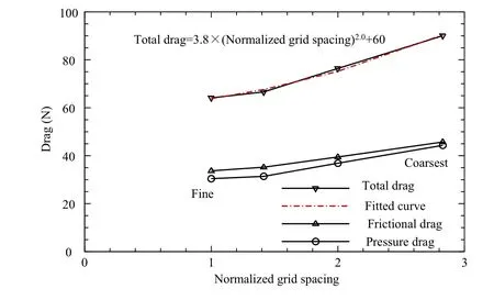
Fig.8 Influence of grid spacing on drag

Figure 4 shows the sectional area of the pod as a function of the longitudinal position.The longitudinal position and area are non-dimensionalized with Lref,for which the pod length for the short model(3.0 m)is used.The sectional area depicted here is not for half of the model but for both sides.To introduce a laminar-turbulent transition in the front part,the axial position of the maximum sectional area for the optimized model(X/Lref=0.42)is located more toward the front side than that of the short model(X/Lref=0.47).

3.2 Computational domain and boundary conditions

The computational domain is shown in Fig.5a.The definition of the axes is as follows:The X-axis lies along the direction of the travel,pointing to the rear side,the Y-axis is the lateral direction,and the Z-axis points upward.The origin of the coordinate system is located at the front of the pod in the X-direction,Y=0 is located at the center of the pod,and Z=0 is the elevation of the floor of the tube,as shown in Fig.5b.Only half of the pod is computed by employing a symmetry boundary condition at the Y=0 plane.The length of the Hyperloop tube is 13.8 m,i.e.,-3.4 m ≤X ≤10.4 m.

3.3 Computational mesh

The computational mesh was made by applying the mesh generation function implemented in the STAR-CCM+code[24].The mesh generation approaches Prism Layer Mesher and Trimmer are used.Trimmer makes a prism or hexahedral cells near the wall region,whereas Prism Layer Mesher generates a cubic mesh in the bulk region.The gap between the meshes of the Prism Layer Mesher and Trimmer is filled with unstructured meshes.

Fig.9 Computational mesh on the symmetry plane for Fine-2

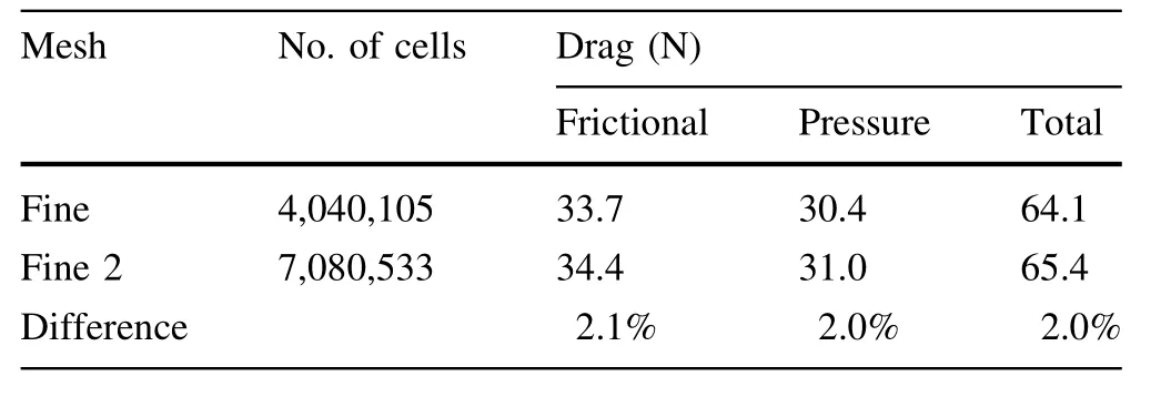
Table 3 Computed drag for the cases with different mesh topology

The surface mesh of the optimized model is shown in Fig.6a.The average surface mesh size in the X-direction is 8.8 mm,which corresponds to 0.25%of the pod length.Note that,according to the guidelines for the Gamma transition model proposed by the developer of the CFD software,STAR-CCM+[21],a mesh length of less than a 0.5%chord is recommended,and we used half the length of the recommendation.The validation case demonstrated by the developer uses a measurement by Somers[25]for NLF(1)-0416 airfoil at Ma=0.1,Re=4×106,and a 4°angle of attack.Nonetheless,a mesh dependency study is described in Sect.4.1 to evaluate the influence of the mesh size on the CFD result.

In the bulk region,four mesh sizes are used.Referring to Fig.6b,the finest cubic mesh of 8.8 mm is used in zone 1 to capture the detailed flow field.The mesh size doubles as the zone number increases, i.e., zone 2 is a cube of 17.7 mm,zone 3 is 35.4 mm,and zone 4 is 70.7 mm.

The computational mesh on the sliced plane at X=1.5 m is shown in Fig.7a.The thickness of the first mesh layer on the wall is 25 μm,and the second layer is 1.5 times thicker than the first layer,i.e.,the growth rate is 1.5.Fourteen layers are generated by Prism Layer Mesher,keeping the growth rate constant at 1.5.The total thickness of the prism layer is 14.5 mm.As shown in Fig.7b,the prism layer is smoothly connected to the bulk region without a noticeable jump in the mesh size.

4 Results of simulations

4.1 Mesh dependency study

Two types of mesh dependency study were performed.The first one was the parametric study for the mesh size,and the second was the study for the mesh topology,i.e.,the dimension of Zones described in Fig.6b was modified.

4.1.1 Mesh size

A mesh dependency study based on grid convergence index(GCI)[26]was conducted for the optimized model to evaluate the influence of the computational mesh on the CFD result.The traveling speed of the pod was set to 125 m/s at a system pressure 0.15 bar and at an inlet air temperature 300 K,which corresponds to Ma=0.36.The Reynolds number based on the body length is Re=3.8×106.Four mesh cases with different mesh sizes were used,as listed in Table 2.The prism layer thickness shown in this table is the thickness of the first layer mesh adjacent to the wall surface.Note that the mesh shown in Figs.6 and 7 corresponds to the fine mesh.

The computed pressure drag,frictional drag,and total drag are shown in Fig.8 as functions of the normalized grid spacing,which is normalized by the fine grid spacing listed in Table 2.As the grid spacing decreases,the drag converges to an asymptotic value.The fitted exponential curve for the total drag is also depicted in Fig.8.The exponent of the fitted curve,which indicates the accuracy of the numerical scheme in space,is 2.0.Because the discretization schemes used for the convection and diffusion terms in the momentum equations and the SST k-ω turbulence model are the second-order accuracy with respect to space, the accuracy at 2.0 is considered reasonable.

4.1.2 Mesh topology

The influence of mesh topology on the drag is investigated in this section.Fine-2 mesh is generated from the fine mesh by changing the dimension of zones.The mesh on the symmetry plane for Fine-2 is shown in Fig.9.Comparing Figs.6b(Fine)and 9(Fine-2),zones 1 and 2 of Fine-2 are prolonged almost to the outlet boundary.The number of cells for Fine-2 increases to seven million due to this modification.The computed frictional,pressure and total drags for Fine-2 are about 2%larger than those for the fine mesh,as listed in Table 3.The fine mesh has been adopted for all further simulations in this work,because of the lower computational cost.

Fig.10 Distribution of Y+on a short and b optimized models

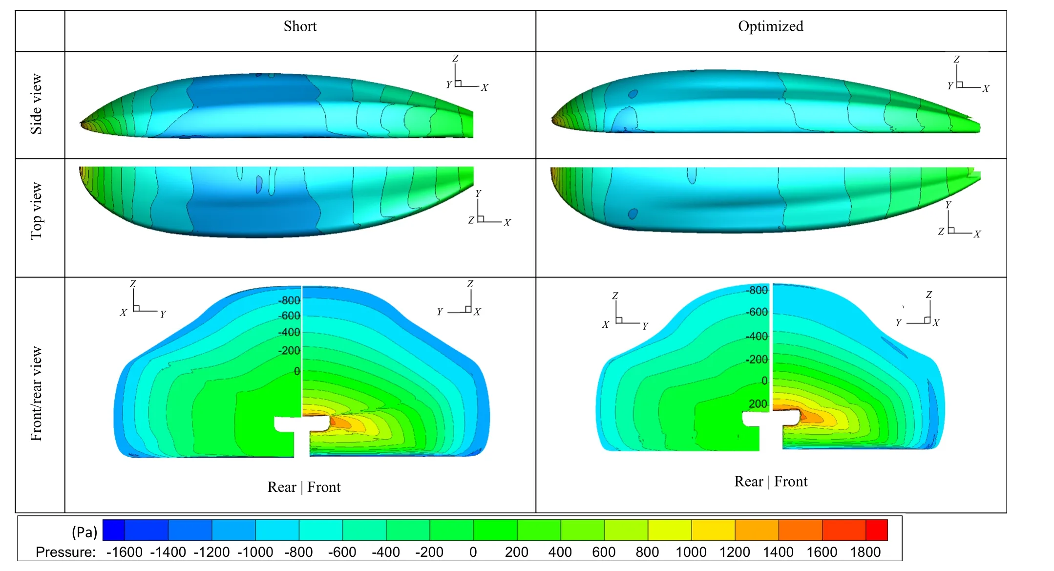
Fig.11 Comparison of pressure distribution on the pod between short and optimized models

Fig.12 Comparison of streamlines at center plane between a short and b optimized models

4.2 Comparison between the two models

In this section,the simulation results are compared between the short and optimized models.The conditions of the simulation are same as those used for the mesh dependency study:The pod speed is 125 m/s at a system pressure of 0.15 bar and an inlet air temperature of 300 K. The parameters for the fine mesh computation were used for the simulation.The computations were continued until a steady state was attained.

The distribution of Y+is shown in Fig.10,where Y+is the non-dimensionalized thickness of the wall-adjacent mesh,which is defined as follows:

where τwis the wall shear stress,μ is the dynamic viscosity,and ythickis the thickness of the wall adjacent cells.Because the wall function is not used in these simulations,it is recommended to use a thinner mesh than 1(Y+≤1)to resolve the viscous sublayer.Figure 10 indicates that such a condition is mostly satisfied.

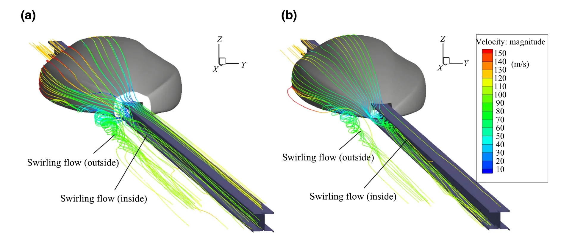
Fig.13 Comparison of streamlines between a short and b optimized models,viewed from the rear side

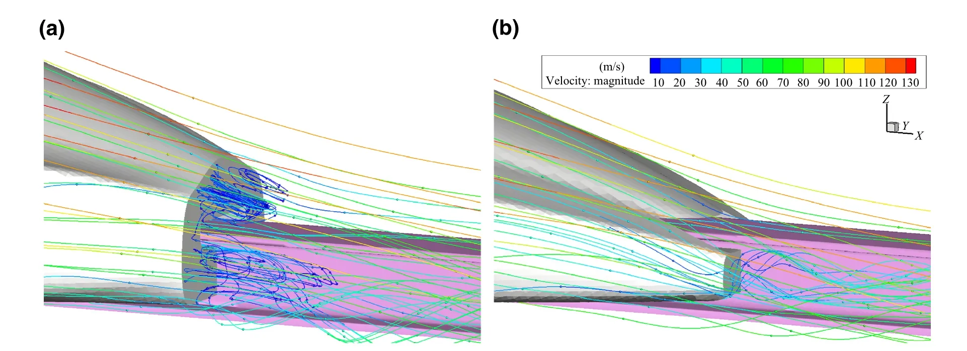
Fig.14 Comparison of streamlines around the rear-end between a short and b optimized models

4.2.1 Drag and lift forces

The computed drag and lift forces acting on the entire pod,i.e.,not half the body,are summarized in Table 4.Here,Fpis the pressure drag,Ffthe frictional drag,and Ftthe total drag,i.e.,Ft=Fp+Ff.The pressure,frictional drag,and total drag coefficients based on the frontal area are defined,respectively,as follows:

where ρrefis the density of air at 0.15 bar.In addition,we define the frictional drag coefficient based on the surface area as

where S is the surface area of the pod listed in Table 1.

Fig.15 Comparison of velocity X distribution on symmetry plane between a short and b optimized models,in m/s.The aspect ratio of Z/X is set to 5

The pressure drag of the optimized model is 30.4 N,which is 24%smaller than that of the short model(39.8 N).Because the frontal area for the optimized model is only 12%smaller than that for the short model(as listed in Table 1),the pressure drag reduction of the optimized model is not only due to the smaller frontal area but also the improved shape.This can be recognized by Cp,which for the optimized model(0.058)is 12%smaller than that of the short model(0.066),as shown in Table 4.

The frictional drag for the optimized model is 33.7 N,which is slightly smaller than that for the short model,i.e.,34.8 N,although the surface area for the optimized model is 10%smaller than that for the short model.The frictional drag coefficient based on the surface area CfSfor the optimized model(2.99×10-3)is 8%larger than that for the short model(2.77×10-3).The reason for this will be discussed in Sect.4.2.3,where the distribution of the skin friction coefficient is visualized.

The total drag for the optimized model is 64.1 N,which is 14%smaller than that for the short model(74.6 N).This drag reduction is achieved mainly by the decrease in the pressure drag and slightly due to the decrease in the frictional drag as mentioned above.

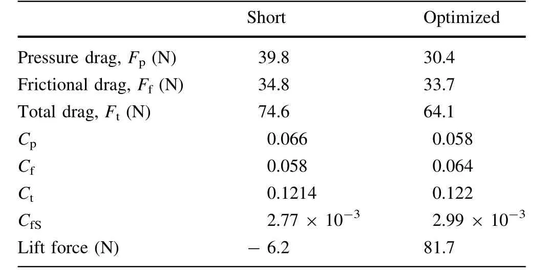
Table 4 Computed drag and lift forces for 0.15 bar

The computed lift force(-6.2 N for the short model and 81.7 N for the optimized model)is an order of magnitude smaller than the pod weight(200 kg),meaning that the pod does not lift off from the ground.

4.2.2 Pressure and velocity field

The pressure distribution on the pod is shown in Fig.11.The pressure given here is the pressure relative to the system pressure(0.15 bar).The maximum pressure appears at the front of the pod,and the maximum values are almost the same between the short and optimized models.The minimum pressure appears at around the midpoint of the pod.Because the blockage ratio of the short model is larger than that of the optimized model,as listed in Table 1,the minimum pressure for the short model becomes lower than that for the optimized model.With respect to the pressure recovery around the rear of the body,the optimized model shows a better recovery than the short model.Referring to the bottom row in Fig.11,the maximum pressure in the rear view for the optimized model is above 200 Pa,whereas that for the short model is less than this value.

The pressure distribution and streamlines on the symmetry plane and pod are shown in Fig.12.The streamlines are smooth in general,and the flow separation is observed only in the region behind the rear end wall of the short model.This result clearly shows that the flow separation does not occur above the both pods,in the region of the reverse pressure gradient.

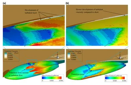
Fig.16 Distribution of skin friction coefficient on pod and turbulent viscosity on the symmetry plane for a short and b optimized models

A three-dimensional view of the streamlines around the pod is shown in Fig.13.Two sets of swirling flows,inside and outside,as indicated in the figure,can be seen for both models.The swirling flow outside is generated from the side wall of the pod where the body width begins to decrease.The swirling flow inside is generated at the rear end of the body,which interacts with the I-beam rail downstream.The swirling flow inside for the optimized model clearly features a counterclockwise rotation,whereas that for the short model is more chaotic because of the larger wake field.

Magnified views of the streamlines around the rear end wall are compared in Fig.14.The flow behind the rear end wall of the short model stagnates,which results in a larger wake field.Meanwhile the streamlines for the optimized model is smoother than that for the short model,and the wake field is consequently smaller.

The wake field is compared in Fig.15.The region where velocity X is lower than 100 m/s in the downstream of the pod is obviously larger for the short model than that for the optimized model.However,the velocity distribution above the rear part of the pod shows a similar feature between the two because the flow separation does not occur in this region,as the streamlines in Fig.12 indicate.

4.2.3 Laminar-turbulent transition

Fig.17 Comparison of limiting streamlines for a short and b optimized models

The location of the transition from laminar to turbulent flow,which is typically prescribed in the CFD simulations,is calculated in our simulations using the Gamma transition model.In the turbulent flow regime,the friction on the wall is higher than that in the laminar flow regime owing to the turbulent viscosity.To visualize the location of the laminar-turbulent transition,the skin friction coefficient on the pod is shown in Fig.16 together with the distribution of the turbulent viscosity on the symmetry plane.Here,the skin friction coefficient is defined as follows:where τwis the wall shear stress,ρrefthe reference density,and U the pod traveling velocity.The laminar-turbulence transition point is emphasized by the dashed line in Fig.16.The laminar flow regime for the short model is apparently larger than that for the optimized model,meaning that the transition for the short model occurs more on the rear side.This is mainly because the maximum sectional area of the short model is more on the rear side than that of the optimized model.However,comparing the skin friction around the downstream of the transition point between the short and optimized models,the skin friction of the short model is higher than that of the optimized model.This is caused by the faster development of the turbulent viscosity for the short model than that for the optimized model,as can be seen in the top row of Fig.16.

The frictional drag coefficient based on the surface area for the optimized model(CfS=2.99×10-3)is 8%larger than that for the short model(2.77×10-3),as listed in Table 4.The lower CfSfor the short model is considered to be resulted from the larger area of the laminar flow regime due to the delay of the transition.

To observe the flow separation specifically,the limiting streamlines are drawn in Fig.17.The flow separation line is indicated with the dashed line.The flow separation occurs at the rear end wall for both models.The flow separation also takes place at the convex part at around the rear of the body for the short model,as shown in Fig.17a,whereas it occurs at the side bottom part of the body for the optimized model,as shown in Fig.17b.Figures 16 and 17 indicate that a flow separation occurs in a turbulent flow,whereas a laminar flow separation is not observed for these models.

4.3 Influence of system pressure on laminarturbulent transition

Three cases of simulation with different system pressures,0.075,0.15 and 0.3 bar,were computed for the optimized model in order to investigate the influence of the systempressure on the laminar-turbulent transition.The traveling speed of the pod was set at 125 m/s for all the cases.The Reynolds number is 1.9×106,3.8×106,and 7.7×106for the system pressure at 0.075, 0.15, and 0.3 bar,respectively.Note that the Reynolds number is almost proportional to the system pressure,because the dynamic viscosity of air is almost constant in this rage of pressure[27],and the density is proportional to the pressure.

Table 5 Drag coefficient for different system pressures

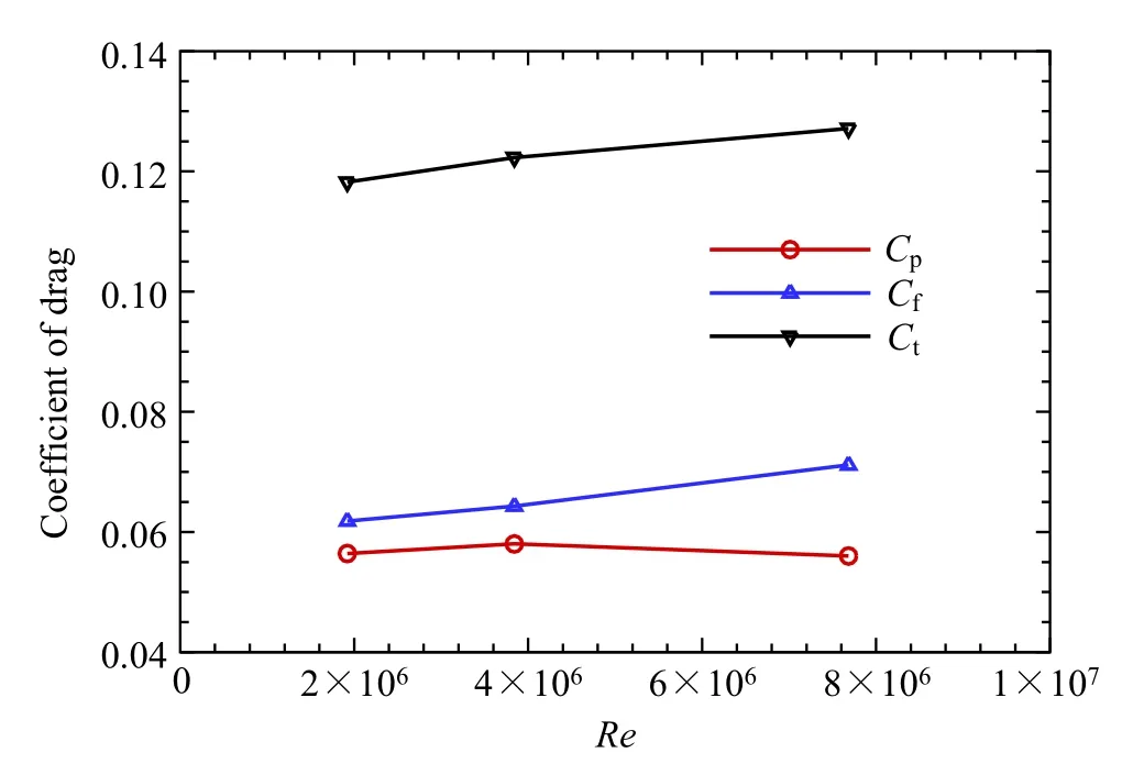
Fig.18 Drag coefficient as the function of Reynolds number

The computed drag coefficients are listed in Table 5.The frictional drag coefficient Cfincreases with the increase of the Reynolds number,as shown in Fig.18.This tendency is typically observed for a flat plate in the transition regime[15].Cffor 0.3 bar is 15%larger than that for 0.075 bar.Meanwhile,Cpdoes not significantly change within the range of the Reynolds number considered here.Consequently,the total drag coefficient Ctfor 0.3 bar is 7%larger than that for 0.075 bar.

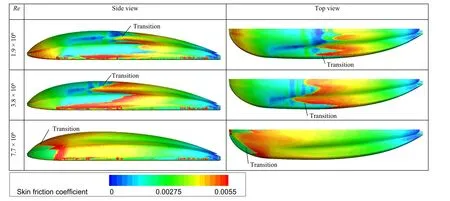
Fig.19 Distribution of skin friction coefficient for different Reynolds numbers

To observe the transition point,the distribution of skin friction coefficient is compared in Fig.19.In this figure,the transition occurs where the skin friction coefficient jumps from a lower value to a higher value.The simulation results clearly show that the transition point moves to the front side as the Reynolds number increases,which is considered to be reasonable from the viewpoint of the critical Reynolds number[28].

5 Conclusions

An aerodynamics analysis was conducted for a Hyperloop pod for the purpose of understanding the laminar/turbulent flow around the pod designed by Swissloop.Because the thrust force of our pod is given by a linear induction motor instead of the propelling of the wheels,the downforce does not play an important role in terms of the acceleration and maximum speed,and thus,we focused on the drag force.Three-dimensional computational fluid dynamics simulations were conducted,with the air being modeled as compressible.The pod length is 3 m when traveling at 125 m/s under a system pressure of 0.15 bar,which corresponds to Ma=0.36 and Re=3.8×106.The novelty of this study is the application of the Gamma transition model,which can predict the laminar-turbulent transition point,to the Hyperloop pod.The shear-stress transport k-ω model is used,but the wall function was not employed to calculate the flow field in the viscous boundary layer.

First, a mesh dependency study was conducted to investigate the influence of the mesh size on the computational result,and the second-order accuracy in space was obtained for the drag force.

Second,we compared the aerodynamic performance of the two representative designs of our pods,namely short and optimized models.The concept of the short model was to delay the laminar-turbulent transition to decrease the frictional drag. Meanwhile, the optimized model was designed to minimize the pressure drag by(1)decreasing the frontal area and(2)introducing the laminar-turbulent transition more toward the front part of the pod in order to avoid flow separation in laminar flows.The transition point was clearly indicated by the jump in the distribution of the skin friction coefficient.The transition of the short model occurred more on the rear side than that of the optimized model,because the maximum sectional area of the short model is more on the rear side than that of the optimized model.This resulted in 8%smaller CfS(frictional drag coefficient based on the surface area)for the short model than that for the optimized model.However,since the surface area of the optimized model is 10%smaller than that of the short model,the frictional drag for the optimized model(33.7 N)was slightly smaller than that for the short model(34.8 N).The pressure drag for the optimized model was 24%smaller than that for the short model,half of which is due to the decrease in the frontal area.The streamlines on the symmetry plane clearly showed that the flow separation did not occur above the both pods,even in the region of the reverse pressure gradient.The smoothed rear end shape for the optimized model resulted in the smaller wake field than that of the short model.Consequently,the total drag for the optimized model was 14%smaller than that for the short model.

Finally,we investigated the influence of the system pressure on the drag coefficient and the transition point through the comparison between three simulation cases at different system pressures: 0.075 bar (Re=1.9×106),0.15 bar(Re=3.8×106),and 0.3 bar(Re=7.7×106).The frictional drag coefficient increases with the increase of the Reynolds number,which is typically observed for the frictional drag of a flat plate in the transition regime.Meanwhile,the pressure drag coefficient is not significantly influenced by the Reynolds number.The transition point moves to the front side as the Reynolds number increases,which is considered to be reasonable from the viewpoint of the critical Reynolds number.

AcknowledgementsThe authors acknowledge all the members of the Swissloop Team for their great endeavor to compete in the Hyperloop pod Competition and to push the Hyperloop technology forward.The authors gratefully acknowledge Connova AG for their support in manufacturing of the pod.

Open AccessThis article is licensed under a Creative Commons Attribution 4.0 International License,which permits use,sharing,adaptation,distribution and reproduction in any medium or format,as long as you give appropriate credit to the original author(s)and the source,provide a link to the Creative Commons licence,and indicate if changes were made.The images or other third party material in this article are included in the article’s Creative Commons licence,unless indicated otherwise in a credit line to the material.If material is not included in the article’s Creative Commons licence and your intended use is not permitted by statutory regulation or exceeds the permitted use,you will need toobtainpermissiondirectlyfromthecopyrightholder.Toviewacopyof this licence,visit http://creativecommons.org/licenses/by/4.0/.