The flow characteristics around bridge piers under the impact of a ship *
2020-04-02YanfenGengHuaqiangGuoXingKe
Yan-fen Geng, Hua-qiang Guo, Xing Ke
School of Transportation, Southeast University, Nanjing 211189, China
Abstract: The complicated flow structure around the pier threatens the safe navigation of ships. This paper studies the mechanism of the flow with a ship around the pier, passing or not passing and with consideration of the interval between the ship and the pier. The flow field model and the moving ship model are constructed by the six degrees of freedom (6DOF) solver combined with the virtual unit immersed boundary method and the level set method, both of which are based on the three-dimensional Navier-Stokes equations.The simulation results show that the ship significantly influences the flow around the pier, increasing the flow velocity by 50% to 140%. Away from the bridge pier, the cross-flow velocity decreases. The cross-flow velocity near the side of the pier also increases but in the opposite direction. The ship is affected by the negative yaw moment because of the reverse cross-flow between the pier and the ship. The size of the ship has an important impact on the extent of the affected flow areas but the velocity distribution is roughly in the same shape. The results show double impacts of ship and pier should be considered when determining the safe area of navigation.
Key words: Bridge pier, flow around cylinder, moving ship model
Introduction
The flow in the bridge area of a channel is doubly squeezed and obstructed by the pier and the ship, which makes the flow structure around the pier extremely complicated[1]. This kind of hydrodynamic phenomenon puts the scour of the bridge pier and the ship force in an unfavorable condition and seriously threatens the stability of the bridge pier and the safety of the ship's navigation. Therefore, the bridge area in the channel becomes accident hotspots[2]. The study of the interaction between the flow and the ship has an important academic value and is of practical significance for the safety and controllability of the ship navigation.
The structural change of the water flow in the bridge area has long been a focus of researches[3]. As observed from the large scale flow in bridge areas, the morphological changes of the flow show a certain regularity[4]. The flow structure around the pier is mainly composed of the front shock wave, the turbulent zone induced by the horseshoe vortex on both sides of the pier, and the turbulence in the wake zone behind the pier. In view of a small scale fluid,one can observe that the structural change of the local water flow is affected by many factors and is so complicated that it is difficult to accurately simulate the subtle process of the water flow change. Most of related researches are through physical experiments and numerical simulations. In physical experiments,the characteristic distributions of the water flow around the pier are measured by the acoustic Doppler velocimetry (ADV) or the particle image velocimetry(PIV)[5]. The PIV is an effective tool to measure the instantaneous two-dimensional flow field and the water surface line of the incoming flow[6]. Johnson and Ting[7]used the PIV to determine the variations of the flow structure at different water levels against the Froude number and the relative water depth. It was verified that the instantaneous velocity field, the turbulence intensity and the average velocity field around the pier on the horizontal and vertical sections are clearly three-dimensional layered[8]. The water areas around the bridge can be divided into the front,the middle and the rear areas of the pier in the longitudinal direction and the characteristics of the flow in different areas are completely different[9].With the development of the information technology,the numerical simulation is widely used due to its high accuracy and simplicity[10]. The research boundary and conditions can be expanded, and more practical factors can be taken into account that were simplified and ignored in physical models. Therefore, the conditions set in the numerical simulations can be more consistent with the actual situation in the real-scale and external conditions[11]. The lattice Boltzmann method was used to simulate the 3-D turbulent flow field around the pier and then to analyze the width of the 3-D turbulent flow around the pier under different inflow and pier type conditions[12].Sakib et al.[13]used a flow-3-D model to determine the real vortex characteristics of the wake area around the pier. The large eddy simulation (LES) method is excellent for cases of high Reynolds numbers and can accurately capture the characteristics of the flow with a low computational cost[14]. Kianejad et al.[15]applied LES to investigate the internal flow structure and the vortex dynamics around a submerged gate. The bridge pier affects the flow structure and directly affects the ship and makes the ship navigation difficult to control.The behavior of the ship passing through the pier is a vital issue to be studied. It is found that some parameters of the ship, like the horizontal drift speed,the drift angle, the track belt width and the drift distance, are related with the cross-flow[16]. The RNG k-ε turbulence model can be used to study the force characteristics of the ship[17]. The distance between the ship and the pier affects significantly the force acted by the flow on the ship[18]. The reasonable adjustment of the interval between the ship and the pier can effectively reduce the probability of the collision between the ship and the pier[19]. With the development of the world economy and industry,large-scale ships more and more become an inevitable choice for the navigation[20]. The ship size is one of the important factors to affect the navigational conditions and the external environments and in turns,the related hydraulic phenomena[21]. However, the cases of ships of different sizes passing through a bridge area were not well studied. The ship and the flow are mutually affected. The complicated and variable flow structures have a great impact on the operation of the ship and the ship also brings about the secondary crushing effect on the flow structure. In two controlled cases with and without the ship passing, the vortex behind the pier is found different in a large area under the influence of the ship. The width of the turbulence is always used to evaluate the effect of the ship on the flow as an indicator[22]. Using the threedimensional boundary grid method, Li et al.[19]proposed that the interaction between the ship and the pier in a channel could be compared to an encounter issue of two ships with different speeds. In view of the interaction of the flow and the ship, the adaptive density mesh was used to simulate the interference between the ship and the turbulence around the pier more precisely[23]. However, there are few studies of the interaction between the ship and the flow in bridge areas. This paper studies the flow characteristics around bridge areas affected by ships.
In order to reveal the flow characteristics around the bridge pier affected by ships, the solution of the 6DOF equation is used[24]. The virtual unit immersed boundary method is combined with the level set method[25]to construct the flow field model and the moving ship model. Several cases are simulated to analyze the distribution of the flow field around the pier in the case of no ship passing and the cases of ships passing at different intervals and with ships of different sizes. The results provide a theoretical basis for the safe navigation in bridge areas.
1. Research methodology
1.1 Governing equations and numerical approach
In fluid dynamics, the continuity equation based on the mass conservation says that the mass flowing into a control body is the sum of the fluid mass flowing out of the control body and the fluid mass increment in the control body.
The incompressible flow around the pier is solved using the computational fluid dynamics (CFD)software REEF3D to simulate the interaction between the flow and the ships. The LES method is used in the establishment of the numerical model of the turbulent flow field. It is a method for simplifying the turbulent flow into the superimposed motion of many vortex combinations with different scales. The average flow is significantly affected by the large vortex. The large eddy is directly solved by the Navier-Stokes equation,and is mainly used to respond to the physical processes in the turbulent flows, such as the turbulent diffusion, the mass exchange, and the Reynolds shear stress changes. At the same time, the sub-grid scale(SGS) model of small vortices is constructed to mainly calculate the sub-lattice-scale stress generated during the dissipation and the modeling process, so as to reflect its effect on the large vortex. Therefore, the filter equation is established to filter the Navier-Stokes equation. The filter equation is

where uiis the velocity in the i direction, xiis the coordinate in the i direction, ρ is the pressure,ν is the coefficient of the dynamic viscosity, ∂ijτ is the sub grid-scale stress.
The Smagorinsky SGS model is used to solve the sub-grid stress, which for the incompressible fluid is

1.2 Discretization method
The construction of the model is mainly based on the finite difference method suitable for simulating the fluid flow, with good parallel performance for the discretization of the governing equation. The finite difference method is mature in theory, intuitive in solving process, good in convergence and highly efficient in parallel calculations. For uniform regular grids, high-order formats can be used to improve the accuracy but they are not conducive for irregular computing domain processing and, therefore, regular difference grids are used there. With this consideration, the ghost cell immersed boundary method is used for the calculation with the structural grid of the complex geometric shape boundary. The solid body with complex shapes is immersed into the flow and the re-meshing or overset grids are avoided. The original shortcomings are thus overcome and the simulations of the flow field model and the ship model are more precise[15,24].
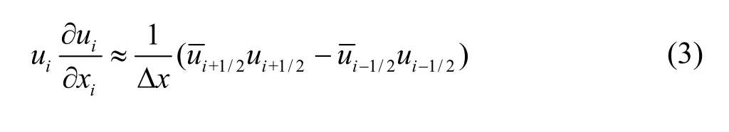
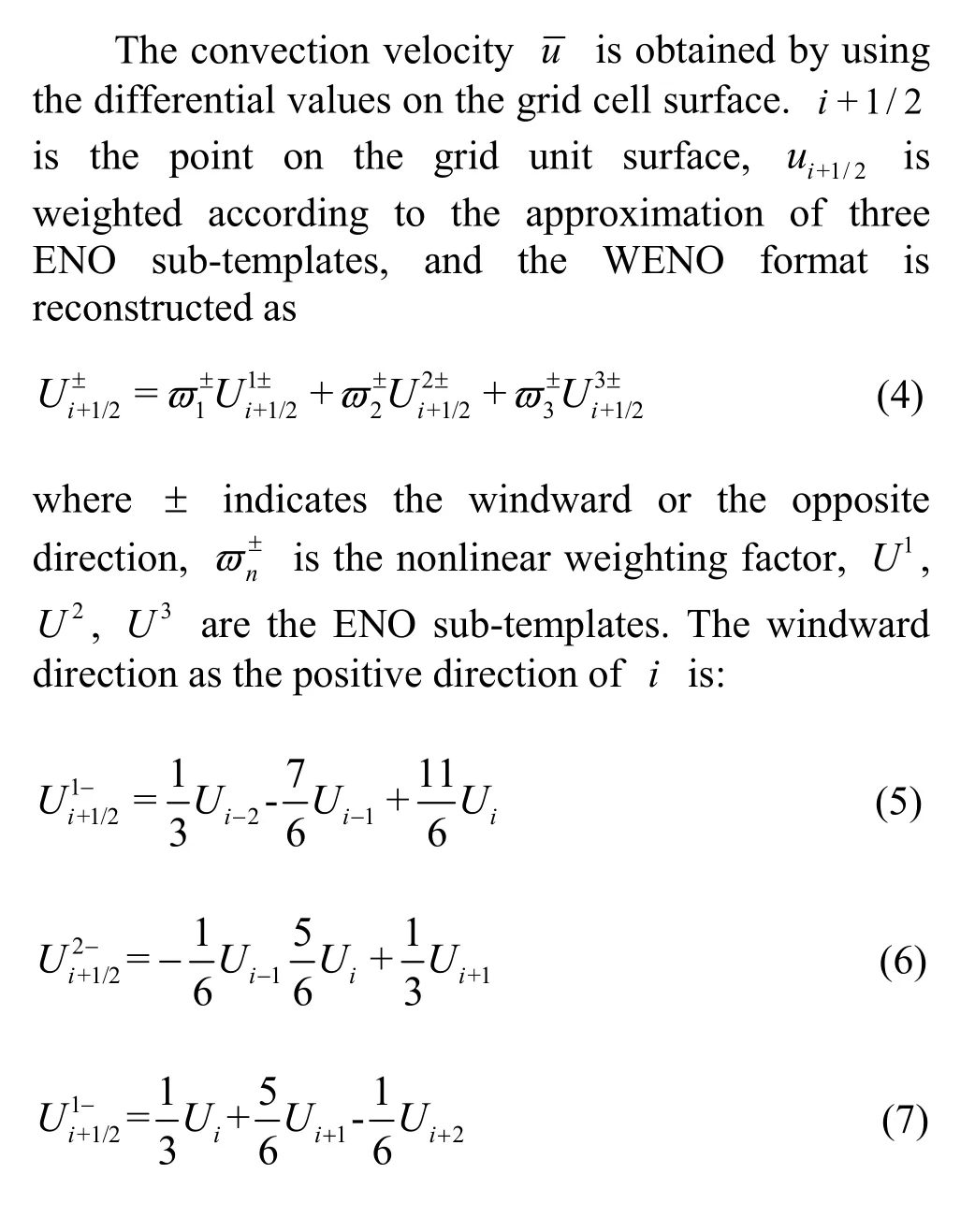
The weighted essential non-oscillation (WENO)format is used in the discretization processing of convective terms[26]. The fifth-order WENO finite difference scheme can handle the high gradient part of the equation solution well by using the local smooth part. The discretization template consists of three ENO sub-templates, which are weighted according to the local smoothness of the discretization function.The better the smoothness, the larger the weight. In the REEF3D, this method is used to discretize the velocity term and the level set function of the convection term in the governing equation, with a high-order accuracy. Meanwhile, the level set method can be used to compute the motion of the interface between two phases and to build a stable fluidstructure interaction model[25]. The dispersion of the turbulent flow energy and the specific energy dissipation rate are discretized by the Hamilton-Jacobi formula in the WENO format. The speed is
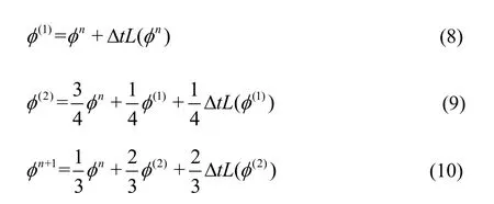
The most complex free surface flow problem can be described by its transient nature. For the time discretization, the third-order Runge-Kutta explicit is used for the time advancement of the momentum and level set equations. The third-order Runge-Kutta explicit equations are:
In order to maintain the stability of the simulation, the number of cells flowing through the unit in a unit time step is kept no more than one, which is called the Courant-Friedrichs-Lewy (CFL) condition.In the three dimensional case, the CFL is
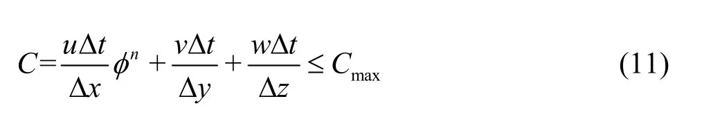
where Cmaxis 0.9.
2. Model setup and validation
The variations of the flow around the pier are analyzed to determine the effective characteristic parameters. A 3-D moving model ship is added to the flow field model with the immersed boundary method to simulate the complex structured grid of the ship boundary. The interaction between the ship and the flow could thus be analyzed. At the same time, six degrees of freedom (6DOF) are given to the model ship to make the movement of the ship more realistic.This process is achieved by the REEF3D.
2.1 Flow field model setup

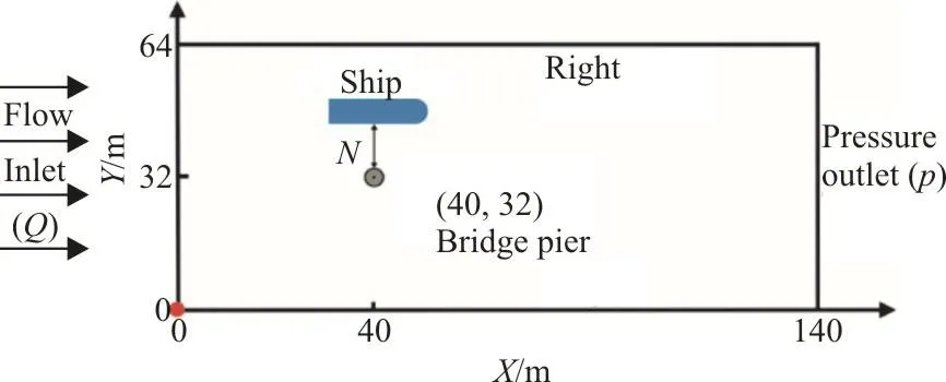
Fig. 1 (Color online) Sketch of the flow field model and boundary condition
2.2 Validation of flow field model
In order to verify the reliability of the basic parameters of the flow field model and the discrete solution method, the simulation results are compared with the available data from previous experiments.Here Melvill’s[27]experiment results are selected as the control prototype. Therefore, the computational domain of the validation model is set the same as the prototype experiment. As shown in Fig. 2, the computational domain of the validation model is a channel with a length of 7.00 m, a width of 1.5 m, a height of 0.35 m and a bottom slope of 0.02%. The pier is located at the center of the channel of a diameter of 0.09 m. The flow in the upstream inlet boundary is set to 0.18 m3/s, the water depth is set to 0.18 m and the flow rate is set to 0.29 m/s. The validation point is set on the X-axis in front of the pier with a distance of 0.20 m away from the pier.
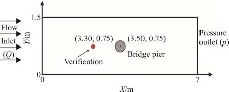
Fig. 2 (Color online) Sketch of the validation domain (m)
Figure 3 shows that the simulated results of vxare comparable with the previous experimental data.The vertical velocity vzis basically the same as the previous experimental data except in the vicinity of the riverbed. The overall data fitting is good, the large error only appears near the riverbed. The reason is that the riverbed in the flow field model is set as the no-slip wall surface and the sub-lattice LES model cannot effectively capture the sudden sweep in the bed surface. Since this paper mainly studies the influence of the interaction between the ship and the flow around the pier, the riverbed is not an important part in the interaction area. Therefore, the large error near the riverbed will not have a great impact on the results.The validation results show that the discrete solution method and the model parameters used in the flow field model is reasonable and reliable. The method and the basic parameters can be used in the simulation analysis.


Fig. 3 (Color online) Verification of longitudinal flow rate and vertical flow rate (m/s)
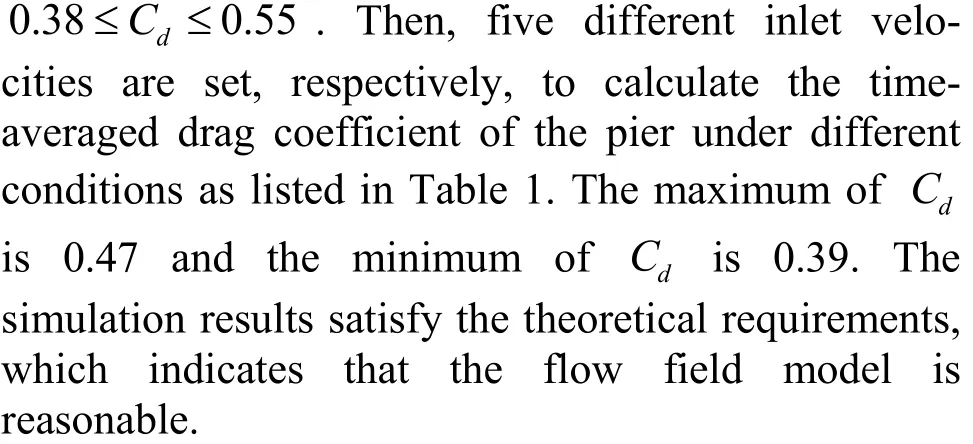

Table 1 Verification of drag coefficient
2.3 Moving ship model
The moving ship model is constructed based on the flow field model to explore the interaction between the ship in the bridge areas and the flow around the pier (Fig. 1). The ship is considered as an entity with 6DOF in fluids. When the flow fluid is stable, the ship is set to start sailing 32 m upstream the center of the pier. The model combines the level set method with the immersed boundary method to describe the interaction on the flow-solid interface.The 6DOF setting achieves a more realistic simulation of the ship movement. Figure 1 shows the positional relationship between the ship and the pier in the moving ship model. Ships of different sizes are used according to different tonnage classes. The ship length is L, the width is W and the depth is H. The draft depth is I. N is the distance from the ship to the pier on the Y-axis.
The distribution of the flow velocity is analyzed around the pier with and without the ship in the inland waterway in the following discussions. In particular,the impact of different ship-pier intervals and ship grades on the water flow is analyzed in detail.Different simulation conditions are listed in Table 2.Three different ship sizes are listed in Table 3. The moment of inertia (J) only depends on the shape,the mass distribution of the rigid body and the position of the axis of rotation. So, it is the exclusive property of different ship grades. It is an important physical parameter to determine the rotation amplitude and the motion variation of the ship when the ship is affected by the external force[15].

Table 2 Calculation conditions
3. Results and discussions
3.1 The flow field around the pier without ship
3.1.1 The mechanism of flow around bridge piers
The 2-D distribution of the flow field around the pier is shown in Fig. 4. The velocity distribution on the free surface on Y-axis of the pier is shown in Fig.5. It can be seen that the influence of the pier on thelocal flow is significant and the flow field changes regularly. Close to the pier, the flow is blocked and the velocity instantaneously decreases. A decelerating flow region is formed in front of the pier. The flow shows vertical stratification characteristics. The local flow is separated into an upflow and a downflow. The upflow is located in the upper layer, approximately between 0.406H and 0.525H in the vertical direction and the downflow is in the lower layer. The separation of the flow generates a local drowning phenomenon (Fig. 6). The flow near the pier is attached to the wall surface. Due to the viscous force of the wall surface of the pier, the flow velocity near the pier is kept within a small range. The flow is separated from both sides of the pier because of the pier’s squeezing action and then a cross-flow region is formed. Compared with the flow velocity near the wall, vxincreases in this area significantly. This area represents the shear and accelerated flow region. The wake region is formed behind the pier where the flow is extremely complicated and is developed into a violent turbulence. Near the pier is a low-speed recirculation zone (Fig. 7).

Table 3 Setting of ship sizes

Fig. 4 (Color online) Snapshot of 2-D distribution of flow field in bridge area

Fig. 5 (Color online) Free surface velocity distribution on the longitudinal axis of a pier
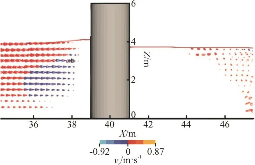
Fig. 6 (Color online) Flow stratification in front of the pier
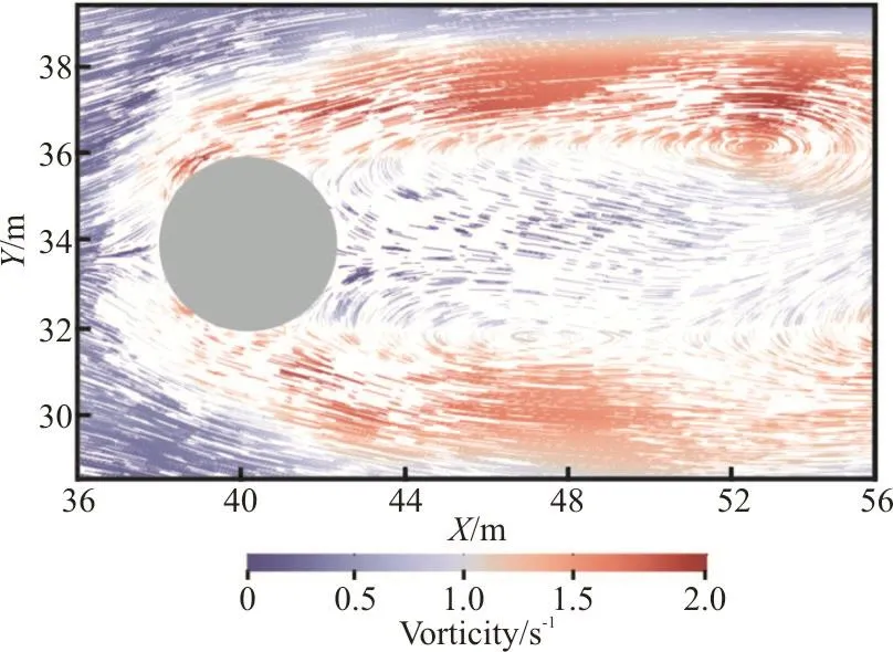
Fig. 7 (Color online) Tail vortex distribution in free surface
At X=60m, the boundary layer separation occurs. The flow velocity drops to a relatively low value and the periodic wake vortex falls off. The wake vortex alternately falls off at the left and right ends of the pier to form the Karman vortex street. The flow velocity gradually increases to the normal flow rate.But as the Karman vortex changes, the longitudinal flow velocity also alternates between positive and negative peaks. The total width of the wake region of the pier is about 3 to 4 times the diameter of the pier.
The streamline trajectory at 0.25H, 0.50H,0.75H and 1.00H (the free level) in front of the pier is analyzed to further reveal the characteristics of the flow movement. As shown in Fig. 8, the vertical velocity component is always generated in the vertical direction when the water flows along the pier’s wall surface. The flow is kept moving downward within a certain range. The same cluster of streamlines flows upward in the wake zone, with the velocity drastically changing with a high frequency, especially near the free surface. Asymmetric wake vortexes are formed at the position of the abrupt velocity change, which indicates that the wake vortexes are the key factor leading to the abrupt velocity change.
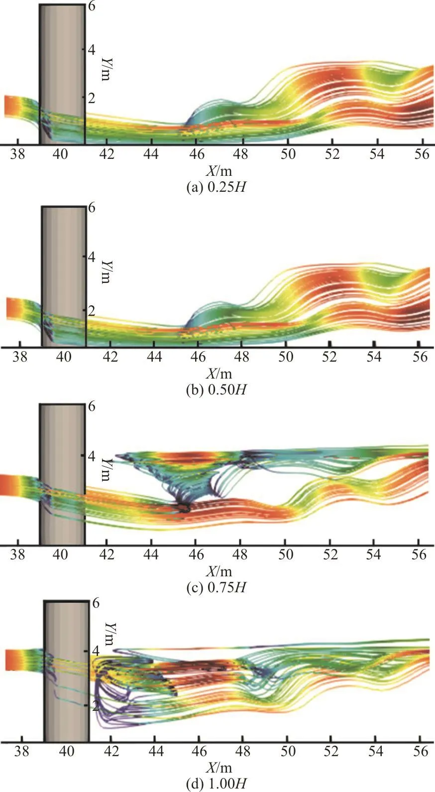
Fig. 8 (Color online) The distribution of streamline at flow surface
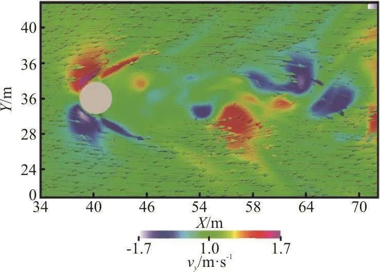
Fig. 9 (Color online) Snapshot of cross-flow distribution around the pier
The cross-flow is the main factor causing the deflection and the torsion of the ship, so the distribution characteristics of the cross-flow around the piers are emphatically analyzed here (Fig. 9). The diversion of the flow in front of the pier forms a distinct cross-flow area, distributed symmetrically along the X-axis of the pier. The peak point of the cross-flow appears before the pier center and the direction generally deflects by 15°-90°. The deflection of the flow in the positive cross-flow area is in the clockwise direction and that in the negative cross-flow area is in the counterclockwise direction. The maximum cross-flow velocity appears in the 45° direction near the wall surface. Within a certain distance behind the pier, the cross-flow is weak in strength. The reason is that the flow downwards to the rear of the pier becomes a free shear flow in the boundary of the near-wake zone but does not enter the near-wake zone.Further in the downstream, the vyis alternately positive and negative. There is a large area of the cross-flow because the vortex street falls off, resulting in the abrupt change of the local cross flow.
3.1.2 The mechanism of flow around bridge piers
The largest water-blocking area around the pier is in the cross section of the pier center, where the flow varies significantly. As shown in Fig. 10, four water depth sections are selected, at 0.25H, 0.50H,0.75H and 1.00H (the free surface), from the bed surface to the free surface.
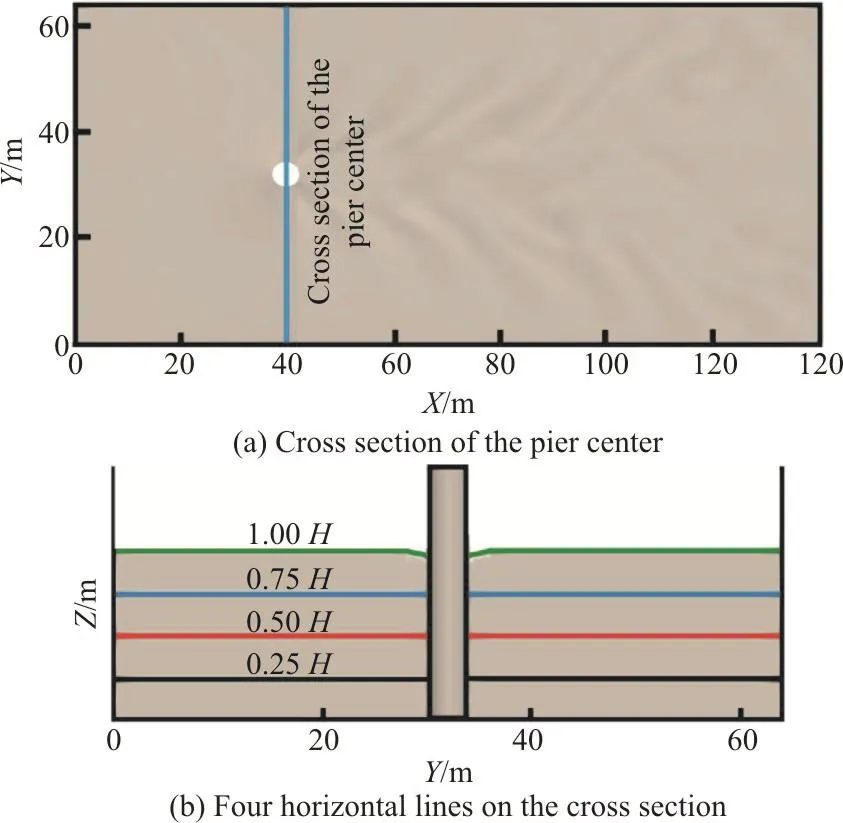
Fig. 10 (Color online) Computational area
The flow velocity distribution on each water depth section is shown in Fig. 11, with the velocity(v) and its components in the X, Y, Z directions. The 3-D flow velocity distribution on both sides of the pier is roughly the same as shown and is symmetrically distributed along the pier. From the center point of the pier to the two sides, the velocity on the different water depth sections increases rapidly at first and then decreases after reaching the peak value. The peaks of v and vxtake roughly the same value, of about 3.8 m/s. The peak of vyis about 0.6 m/s and that of vzis about 0.27 m/s. The distribution of vzis not completely symmetrical as the components in other directions. The peaks on the free surface are not equal and the flow velocity reduction curves on both sides of the liquid surface are asymmetrical, because the vortex shedding in the wake region behind the pier causes the water flow to fluctuate within a certain range close to the pier.

Fig. 11 (Color online) Vertical distribution without ship influence
To consider the influence of the bridge pier flow on the navigation of ships, vywas used to evaluate the safe area of the ships as they pass over the pier area in many studies. The navigation standard of the inland waterway in China takes the cross-flow velocity of 0.3 m/s as the criterion for determining the width of the turbulence. As seen in Fig. 11, the distribution of the flow velocity in Y-axis direction is symmetrical. Based on the cross-section of the pier center, the value of vyat the place about 6 m(1.5D) from the center of the pier is 0.3 m/s.Therefore, the 1.5D area on both sides of the pier is the safe area of the ship navigation, as defined in the standard.
3.2 The flow field around the pier with ship
3.2.1 The interaction mechanism of ship and pier
When the ship approaches the pier (Fig. 12(a)),the ship’s squeezing effect on the water flow creates a low velocity flow zone in front of the ship. As the ship passes along with a part of the water, the blocking effect of the pier decreases the flow velocity. The flow between the pier and the ship is squeezed to generate a water pressure, so the flow velocity near the side of the pier is smaller than those on the other sides.
When the ship passes through the pier center (Fig.12(b)), the flow around the pier is deflected toward the wake region. Due to the increase of the local flow velocity and the formation of the wake vortex, a negative pressure zone is formed somewhere in the rear part of the pier. Then the ship is subjected to a clockwise negative yaw moment. The narrow zone between the ship and the pier will increase the flow velocity, thereby increasing the negative yaw moment and reaching a negative peak when the ship’s gravity center passes over the pier center[28]. Due to the deflection and extrusion effect of the ship, the recirculation zone behind the pier assumes an asymmetrical distribution. The flow width near the ship increases but the longitudinal distance of the recirculation decreases. The recirculation vortex on the other side is narrowly distributed and the turbulent width increases.
When the ship passes away from the pier (Fig.12(c)), the stern enters the negative pressure zone at the rear of the pier, causing the stern to be attracted to the pier side. At the same time, due to the diversion caused by the deflection of the ship, the water quickly flows through the zone between the stern and the pier and then pours into the wake region of the pier. Thus the wake vortex near the ship side is formed in advance and the alternating frequency of the vortex in the wake region increases. The ship is subjected to a counterclockwise positive yaw moment.
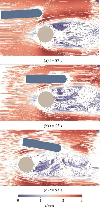
Fig. 12 (Color online) The flow structure and flow velocity distribution around the pier when ship passing
3.2.2 Influence of the intervals (N)
According to the width of the turbulence mentioned above, three different intervals between the ship and the pier are set as 0.5D, 1.5D and 3.0D.The interval N=1.5D means that the ship is in the position where the turbulence width takes the critical value. Based on the size of the 300t ship, the length of the ship is 10.0 m, the width is 2.0 m and the depth is 1.6 m. The draft depth of the ship is 0.6 m. Different simulation conditions are shown in Table 1. Here, the four flow levels of the central cross-section of the pier are taken as the benchmark, which are 0.25H,0.50H, 0.75H and 1.00H.
Figure 13 shows the flow velocity distribution in each flow level when N=0.5D, 1.5D and 3.0D.Compared with the cross-sectional flow velocity without ship passing, the overall variation trend is similar but the sudden change always occurs in the area where the ship passes. v at the ship’s position is rapidly reduced. vyalso decreases rapidly and even becomes negative. After comparison, it is found that the position of the sudden change of the flow rate is basically the same as the position where the ship passes.
When N=0.5D, the changes at 0.25H,0.50H are consistent with those without the ship impact and no sudden change occurs. v changes little but vyincreases greatly. At 0.75H, 1.00H,the ship has a significant influence on the flow velocity. When N=0.5D, the flow velocity is greatly reduced. The flow velocity reduces by 22% at the free level and by 11% at 0.75H. It indicates that the free surface is more easily affected by the ship.vyincreases greatly at 0.75H and the free surface,which is basically between 50% and 140%. However,vyalways reduces to 0 and becomes negative at the position of ship passing. vyis negative by 107% in magnitude but quickly returns to positive values. This is because the ship has a transient impact on the surrounding flow, causing the flow near the side of the pier change its direction, while vyon the other side increases. After the ship passing, the flow returns to the original speed and distribution. Similarly, when N=1.5D, 3.0D, v abruptly change at the position of ship passing. The velocity at other positions does not change much. vyincreases by 100%, 40%,respectively, in the opposite direction to the side of the bridge when N=1.5D, 3.0D. The flow velocities at other positions increase and the increase at the free level is less than that at 0.75H, 0.50H.
Figure 14 shows the changes of the ship’s yaw moment at different intervals between the ship and the pier. The horizontal axis is the downstream direction of the flow and the vertical axis is the direction of the ship’s yaw moment. When N=1.5D, the yaw moment assumes three distinct peak points near the pier. The first positive peak occurs when the ship approaches the pier. The negative peak point appears when the ship passes through the pier center. The second positive peak point appears when the stern leaves the pier. The peak points pose a relatively great risk for the navigation safety. On the contrary, the yaw moment is relatively stable when N=1.5D, 3.0D during traveling. N=1.5D is basically the threshold point for the safety and the risk of the ship navigation.According to the change of the yaw moment, it is relatively safe for the ship passing through the areas with the cross-flow velocity of less than 0.3 m/s.
3.2.3 Influence of ship sizes
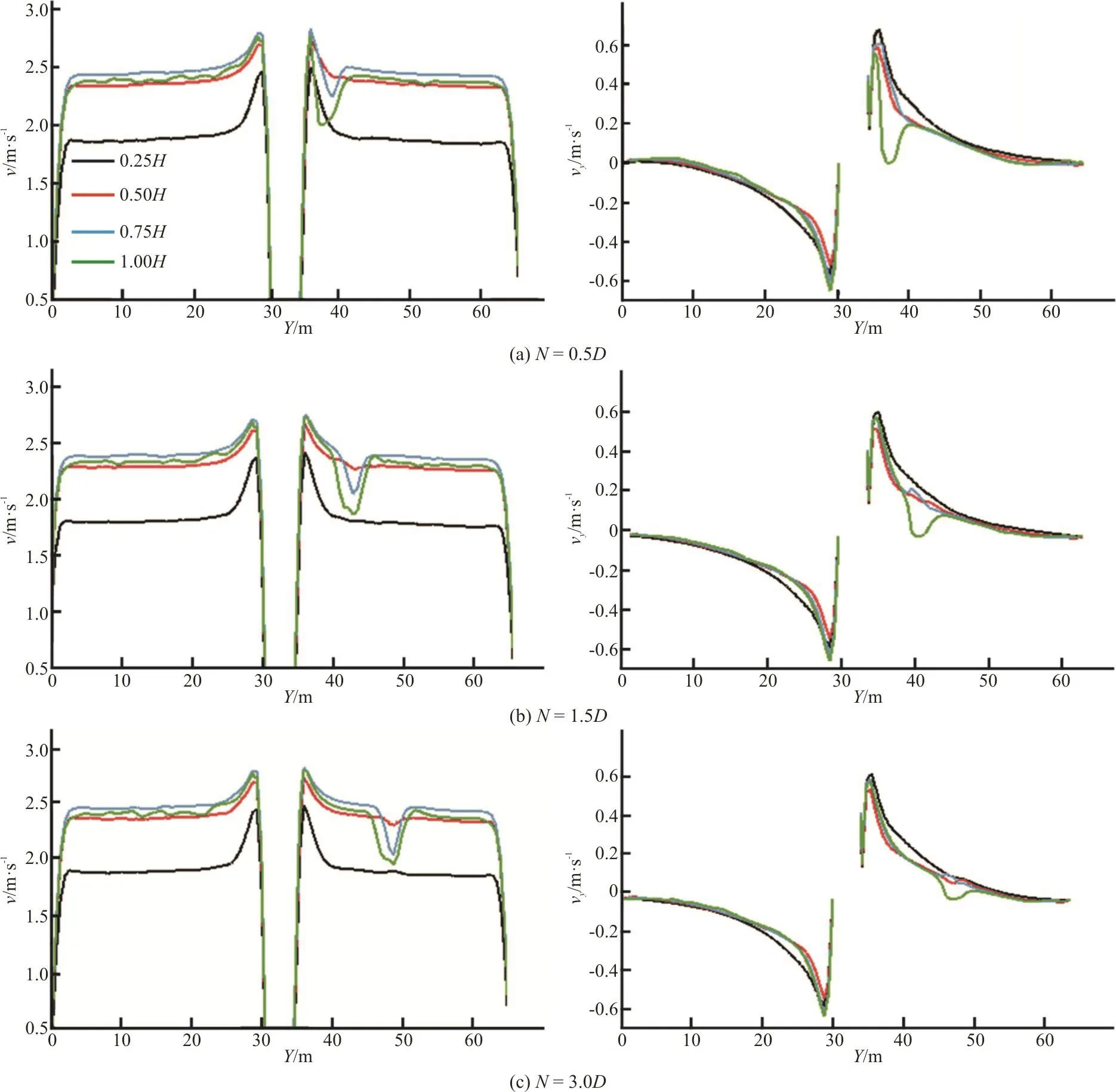
Fig. 13 (Color online) The distribution of the velocity (v) and the Y-axis velocity (vy) induced by the ship (300t) at specified intervals (N)

Fig. 14 (Color online) Ship’s yaw moment (inflow velocity is 2 m/s)
To verify the impact of different sizes of the ships on the flow, the ships with a load of 300t,500t and 800t are used as the simulation prototypes. Three different sizes of ships are listed in Table 2. The 300t ship simulation results have already been analyzed above.

Fig. 15 (Color online) The distribution of the velocity (v) and the Y-axis velocity (vy) induced by the ship (500t) at specified intervals (N)
Figures 15 and 16 show the flow velocity distribution in each flow level when N=1.5D, 3.0D for different ship sizes. Compared with their influence on the flow with that of the ship load of the 300t, the distribution of the flow velocity has some common characteristics. The maximum v near the pier in different cases are all about 2.7 m/s on the free surface.The minimum always occurs where the ship is passing and the value is about 1.9 m/s on the free surface.However, the ship size directly affects the extent of the affected area, including the flow width and depth.As the size of the ship increases, the affected flow area increases. The widths of the flow area affected by the 300t, 500t and 800t ships are 3 m, 5 m and 6 m, respectively. Due to the draught depth of the 500t, 800t ships is larger, the flow velocity at the liquid level of 0.50H is also slightly affected. Meanwhile, different sizes of the ship have a consistent effect on vy. When the ship passes by, vyon the free surface drops to zero instantly, which is common for different cases. But as the ship size increases, the affected areas become much wider. The ship with a load of 500t has a 40% larger flow width as compared with the load of 300t. Meanwhile, the ship with a load of 800t has a 25% larger flow as compared with the load of 500t. According to the comparison of different cases, the farther away from the bridge pier, the smaller the vybecomes. For the ship with the same load, the ship with N=0.5D increases the flow width by 27% as compared with that of the ship with N=1.5D and by 36% as compared with that of the ship with N=3.0D.
Although the affected areas vary when different ships sail at different intervals, the peak values of the velocities in X, Y, Z directions are relatively consistent. It indicates that the ship navigation is less affected by the ship sizes, especially when the load classification of the ship is within 500t.
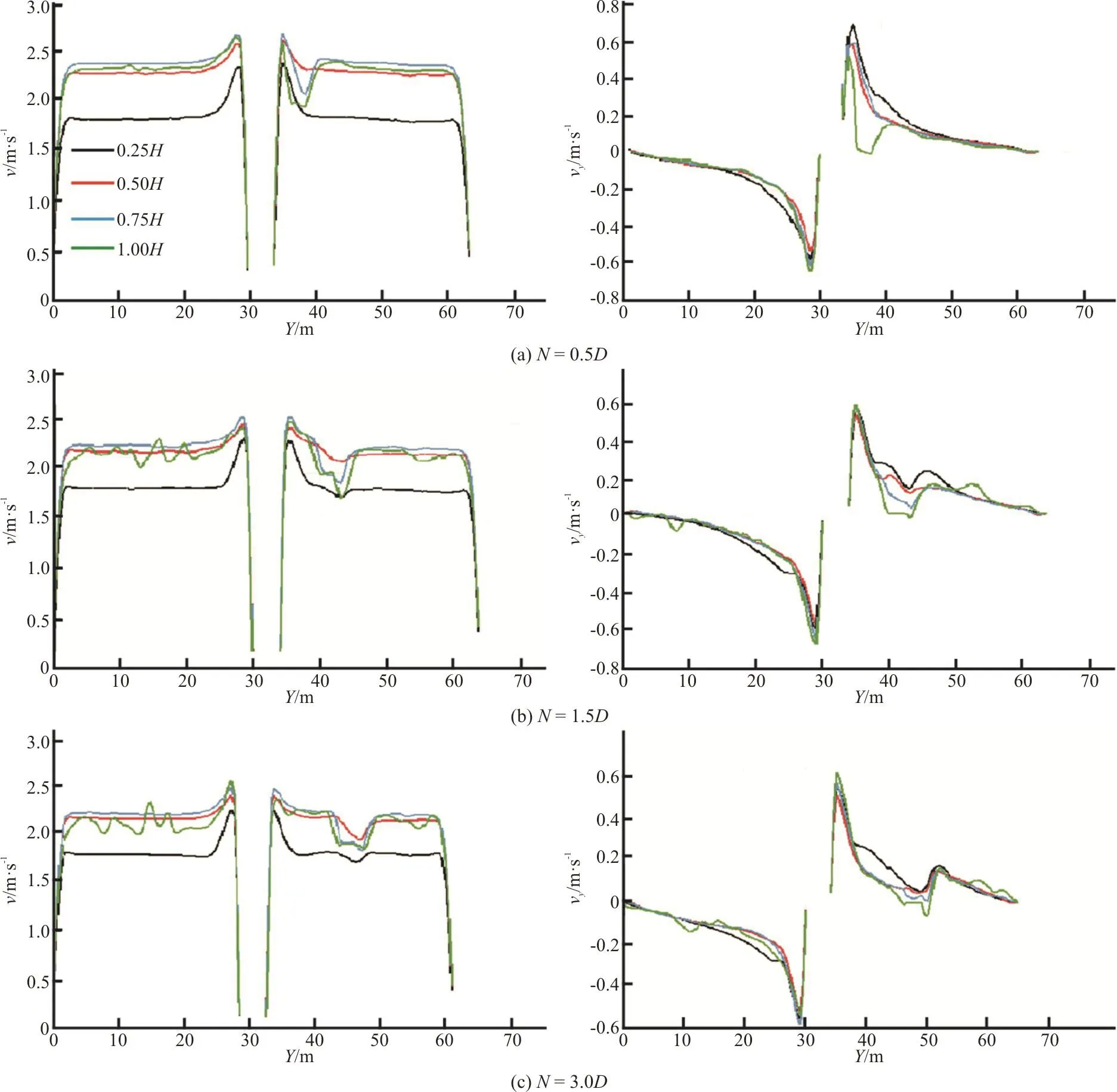
Fig. 16 (Color online) The distribution of the velocity (v) and the Y-axis velocity (vy) induced by the ship (800t) at specified intervals (N)
4. Conclusions
Based on the theory of the 3-D Navier-Stokes equations, the flow field model and the moving ship model are constructed by the 6DOF solver combined with the virtual unit immersed boundary method and the level set method. The distribution of the flow field around the pier is analyzed under the condition of no ship passing and of the ship passing with different intervals.
Compared with the no ship passing cases, the ship and the flow interact with each other. In a certain range near the ship, the flow is subject to twice squeezing. At different intervals between the ship and the pier, the flow velocity and the longitudinal flow velocity increase greatly. But the cross-flow velocity near the bridge pier increases in the opposite direction.The farther away from the bridge pier, the smaller the increase of the reverse cross velocity. Correspondingly, the flow around the pier has a great impact on the ship behavior and it threatens the safety of the ship.
The ship sizes have a major impact on the extent of the affected flow areas. In terms of the width of the affected water flow, the ship with a load of 500t is 40% more affected than that of 300t. The ship with a load of 800t is 25% more affected than that of 500t. The trend of the velocity distribution is roughly the same in different cases. Different sizes of the ship have a consistent effect on the velocity. The ship navigation is less affected by the ship sizes,especially when the load classification of the ship is within 500t.
Overally, the safe distance between the ship and the pier is affected by many factors. It is not sufficient to only consider the influence of the pier. The interaction of the ship and the flow also increases the width of turbulence and threatens the safety of the ship.
杂志排行

水动力学研究与进展 B辑的其它文章
- The effects of caudal fin deformation on the hydrodynamics of thunniform swimming under self-propulsion *
- Control of water contamination on side window of road vehicles by A-pillar section parameter optimization *
- Numerical simulation of the effect of waves on cavity dynamics for oblique water entry of a cylinder *
- Reduction of wave impact on seashore as well as seawall by floating structure and bottom topography *
- Applying physics informed neural network for flow data assimilation *
- Experimental analysis of tip vortex cavitation mitigation by controlled surface roughness *