GENERALIZED FRACTAL LACUNARY INTERPOLATION WITH VARIABLE SCALING PARAMETERS BASED ON EXTRAPOLATION SPLINE

HE Shang-qin FENG Xiu-fang

(1.School of Mathematics and Statistics, NingXia University, Yinchuan 750021, China)

(2.College of Mathematics and Information Science & Technology,Hebei Normal University of Science & Technology, Qinhuangdao 066004, China)

Abstract: In this paper, the generalized Birkhoff (0,m) lacunary interpolation problem for the fractal function with proper perturbable parameters is investigated.An extrapolation algorithm is proposed to obtain an approximate spline polynomial solution, and convergence estimates are presented under the assumption ofThe numerical results show that the interpolate perturbation method we provide works effectively.

Keywords: extrapolation spline; fractal function; lacunary interpolation; scaling factor;approximation order

1 Introduction

Spline interpolation is often preferred over polynomial interpolation, because the interpolation error can be made small even when using low degree polynomials for the spline[1–3].Many research results were obtained about spline lacunary interpolation, such as,spline (0,2,3) and (0,2,4) lacunary interpolation [4], Varma’s (0,2) case of spline [5]and the minimizing error bounds in lacunary interpolation by spline for (0,1,4) and (0,2) case given by Saceed [6]and Jawmer [7].

A fractal is a detailed, recursive and infinitely self-similar mathematical set in which Hausdorff dimension strictly exceeds its topological dimension [8].Fractals exhibit similar patterns at increasingly small scales [9].If this replication is exactly the same at every scale, it is called a self-similar pattern [10, 11].Fractal was widely used as a research tool for generating natural-looking shapes such as mountains, trees, clouds, etc.There were increasing researches in fractal functions and their applications over the last three decades.Fractal function is a good choice for modeling natural object [12], and fractal interpolation techniques provide good deterministic representations of complex phenomena.Barnsley[13]and Hutchinson [14]are pioneers in terms of applying fractal function to interpolate sets of data.The fractal interpolation problems based on Hermite functions and cubic spline are solved in ref.[15]and ref.[16].Viswanathan [17]gave the fractal spline (0,4) and (0,2)lacunary interpolation, and Viswanathan [17]also did research on the fractal (0,2) lacunary interpolation by using the spline function of ref.[5].Inspired by their research, this paper devoted to research the general fractal (0,m) lacunary interpolation with the scaling factors based on the extrapolation spline.

The paper is organized as follows.In Section 2, by using extrapolation algorithm we deduce the explicit formulas of generalized (0,m) lacunary interpolation spline function.The error estimate is also given and numerical example is presented to demonstrate the effectiveness of our proposed method.In Section 3, we use the spline function which has been obtained in Section 2 to interpolate the fractal function.We find that when scaling factors fulfillthere is fractal functionApproximation orders for the proposed class of fractal interpolation and their derivatives are discussed.Numerical simulations are also carried out to show the validity and efficiency of our proposed method.The concluding remarks are given in Section 4.

2 Spline (0,m) Lacunary Interpolation

In this section, the spline explicit formula for the (0,m) lacunary interpolation function is constructed by using extrapolation algorithm.The method we adopt is similar to those given in literature [19].An example for illuminating the details and efficiency of the procedure is provided, and the error estimate will be shown in Theorem 2.2.

2.1 Spline Lacunary Interpolation

For a given partition ∆ : x1< x2< ··· < xN,xk+1− xk= hk, I = [x1,xN], and real values

We define the spline function S∆(x) in each subinterval such that

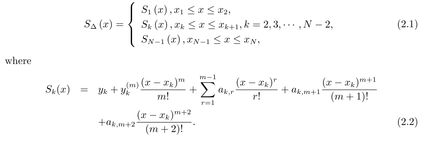
S∆(x) has the following conditions

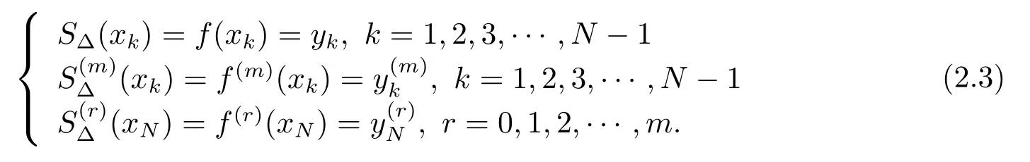
and satisfying

The coefficients of these polynomials can be determined by the following conditions

For k =1,2,··· ,N − 1, we denote

To obtain the unknown coefficients ak,j(k =1,2,··· ,N −1,j =1,2,··· ,m+2,jm),we take the following five steps

Step 1For k =N −1, we have

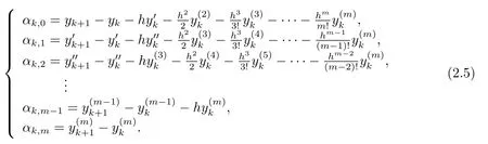
Step 2Solving the equation systems of Step 1, we obtain

where r =1,2,··· ,m − 1;s=m+1,m+2.

Step 3For k =1,2,··· ,N − 2, establishing the equations systems

Step 4Combinating the equations of αk,0and αk,min Step 3, we obtain

Step 5Solving the rest parts of Step 3.

The solutions from step 4 will be substituted by the remaining equations ak,m+1,ak,m+2,starting with+ ···.In view of the coefficient matrix of the equation systems (2.6) is non-singular, thus the unknowns aN−1,1,aN−1,2,··· , aN−1,m−1be solved and obtained.Repeating above iteration, all undetermined coefficients of S∆(x)can be calculated.Therefore, we obtain the following conclusion for spline (0,m) Birkhoff interpolation problem.

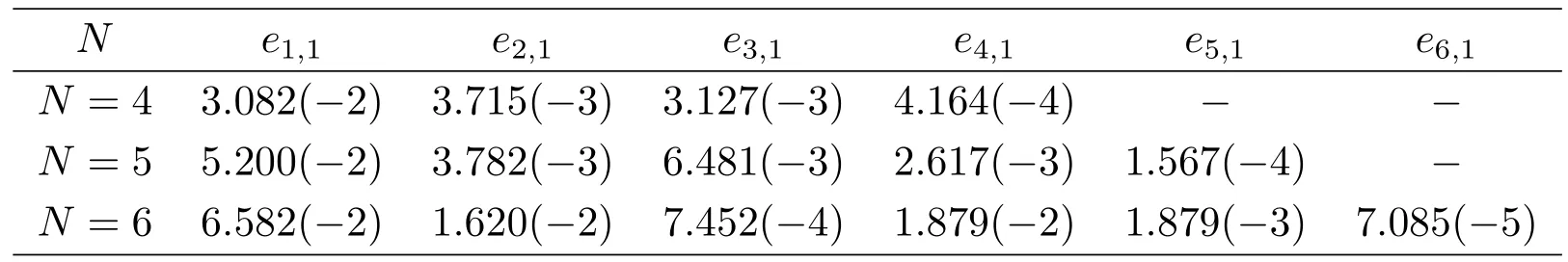
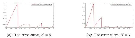
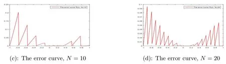
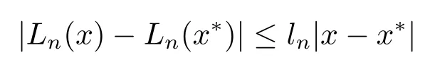
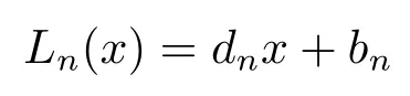
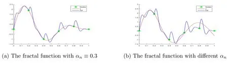
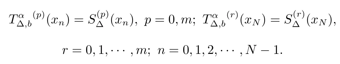
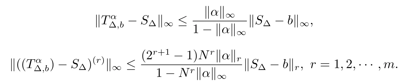
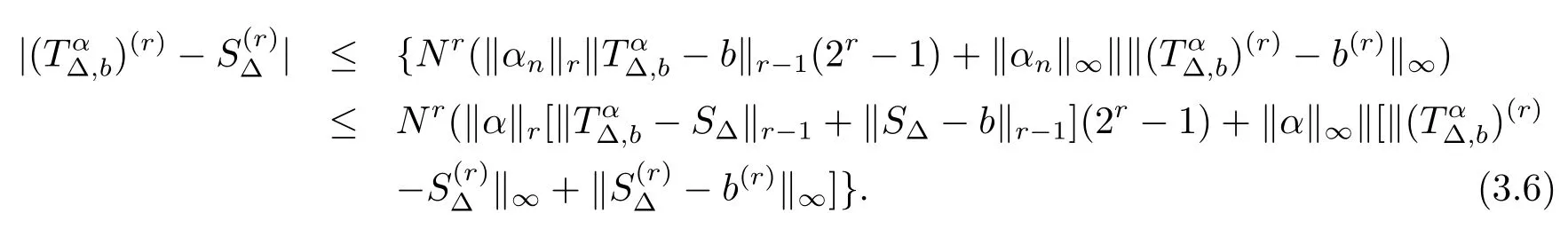
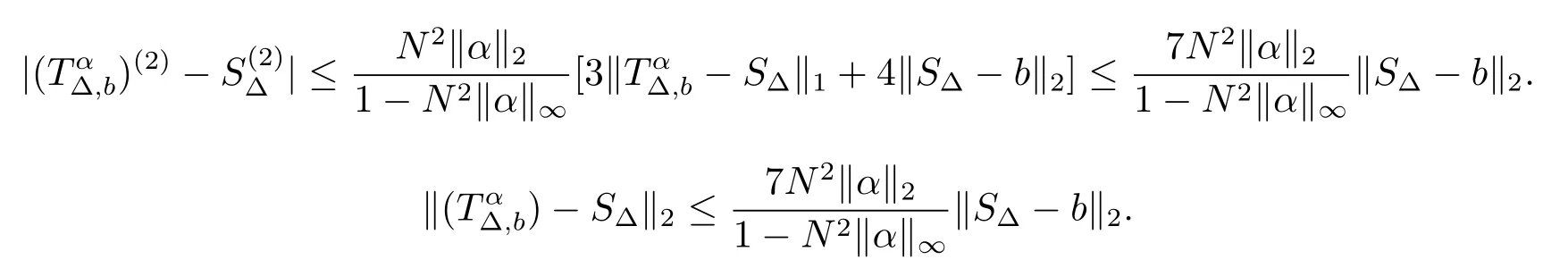
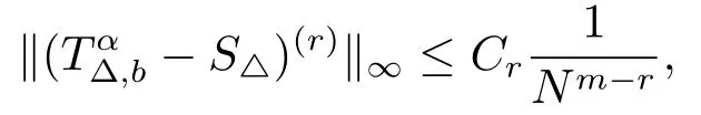
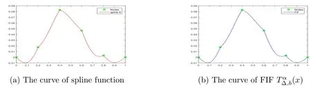
Theorem 2.1Assume that f(x) ∈ Cm(I).For a uniform partition ∆ :={x1,x2,··· ,xN:xk

2.2 Approximation Theory

From the Theorem 2 of ref.[20], we can get the following approximation theory.

Theorem 2.2Assume that f(x) ∈ Cm[−1,1], S∆(x) is the (0,m) lacunary spline function defined by eq.(2.1).When 0 ≤ r ≤ m and −1 ≤ x ≤ 1, we have

where C is constant independent of= max{|f(x)| :x ∈ [−1,1]}, w(f(r),δ) = max{|f(r)(x1)− f(r)(x2)| : |x1− x2| ≤ δ} is the maximum norm modulus of continuity of f(r)(x) on the interval [−1,1].

2.3 Numerical Example

Assume f(x)=x ∗ cos(x)− sin(x).For a uniform partition ∆ :={x1,x2,··· ,xN:xk

Table 1 The absolute error ek,p

Figure 1 The error curve of R(x)=f(x)−S∆(x)

Figure 2 The error curve of R(x)=f(x)−S∆(x)

3 Fractal (0,m) Lacunary Interpolation

For positive integer N >2,consider a data set{(xn,yn)∈R2:n=0,1,2,...,N},where x0< x1< x2< ··· < xN.Let I = [x0,xN], In= [xn−1,xn], n ∈ J = {1,2,··· ,N} and Ln:I →Inbe homeomorphic affinities such as

for all x,x∗∈ I and 0 ≤ ln<1.

Consider N − 1 continuous maps Fn:I × R → R satisfying the following conditions

for all x ∈ I,y,y∗∈ R, and for some 0 ≤ rn<1.

Defining functions wn: I ×R → In× R ⊆ I × R, wn(x,y)=(Ln(x), Fn(x,y)), n ∈ J.The{I×R, wn: n=1,2,...,N}is called an Iterated Function System(IFS)[13].From ref.[17], we know that the IFS has a unique attractor G(g) which is the graph of a continuous function g : I → R satisfying g(xn) = yn(n = 0,1,2,··· ,N), and function g is the fixed point of the Read-Bajraktarevi(RB) operator T :Cy0,yN(I) → Cy0,yN(I) defined

The above function g is called Fractal Interpolation Function(FIF)corresponding to the data{(xn,yn): n=0,1,2,··· ,N} and it satisfies

For a partition ∆ := {x0,x1,x2,··· ,xN: xn−1< xn,n ∈ J} of I = [x0,xN], xn−xn−1:= hn, and the data set {(xn,f(xn)), n = 0,1,2,··· ,N}, suppose that Fn(x,y) =αn(y −b(x))+f(Ln(x)),where αnis called scaling factors,satisfying|αn|<1,and b:I → R is a continuous function, such as b =f, b(x0)=f(x0), b(xN)=f(xN).

Thus,we ensure the existence of a fractal function(Tf)(xn)=f(xn)(n=0,1,2,··· ,N).From (3.1), we can obtain

The most widely studied functions Ln(x) so far are defined by the following,

with

In many cases, the data are evenly sampled h=xn− xn−1,xN− x0=Nh.

Example 1Consider function f(x)=(2x2−5x+3)sin(10x).For a uniform partition∆ := {x0,x1,··· ,x6: xn−1< xn,n = 1,2,··· ,5} of [0,1]with step sizex2f(x).The left graph of Figure 3 shows the fractal function with αn=0.3(n=1,2,··· ,5).The right graph presents the fractal function with scaling variable

3.1 Interpolation Theorem

We denote α =(α1,α2,··· ,αN),

Figure 3 y =(2x2 −5x+3)sin(10x) with N =5

Theorem 3.1Assume that f ∈ Cm(I), ∆ := {x0,x1,··· ,xN: xn−1< xn,n ∈ J}be an arbitrary partition of I = [x0,xN].There are suitable smooth functions b and αn,when scaling factors αnfulfilthe corresponding fractal functionsatisfies

with boundary conditions,

ProofFor convenience, in the following k = 0,1,2,3,··· ,N − 1.Let S∆(x) be prescribed in eq.(2.1), we choose smooth function b ∈Cm(I) to satisfy

Consider the operator T :Cm(I)→Cm(I)

We can deduce that

Using the conditions on b and the properties Ln(xN) = Ln+1(x0) = xn(n ∈J) of Ln, we obtainfor r = 0,1,··· ,m. From (3.2) and (3.3), we get

For f,g ∈ Cm(I), r =1,2,··· ,m, x ∈ In, we have

When r =0,

It is apparently seen from the above discussion that

3.2 Approximation Estimates

we will give error estimates forand obtain convergence results while choosing suitable perturbation parameter αn.Consider I =[0,1],0=x0

Theorem 3.2For the uniform equidistance partition of I =[0,1],the following bounds for the fractal function and its derivatives hold:

ProofFrom the equationIn, n ∈J, we have

Then

It’s evident that the following equality holds

Therefore, we have

It can be easy deduced that

When r =1, using (3.7) and (3.5), we have

Similarly, when r =2, we obtain

Summarizing the above process, we can obtain the result.

Theorem 3.3Assume that f ∈Cm([0,1]).is the fractal interpolation function given in Theorem 3.1.For uniform equidistance partition on [0,1], when the scaling factor αnsatisfiesr =0,1,··· ,m, we have

as N → ∞,r =0,1,··· ,m.

ProofUsing the triangle inequalityand from result of ref.[17], for n ≥ j, k = 0,1,2,··· ,j,we have

here Cris the constant only dependent on r.

Example 2Taking m = 2, consider function f(x) = (2x2−4x + 3)N(sin(x))N,b(x) = cos(x)f(x), and the uniform partition of [0,1], ∆ : 0 = x0< x1< ··· < xN= 1 with step h = xn− xn−1= 1/N,n = 1,2,··· ,N, S∆(x) is the spline function defined by eq.(2.1).We only consider N = 5, and take scaling vector α1= 0.01x, α2= 0.005x2,α3= 0.01(x − sin(x)), α4= 0.01 sin(x),Obviously, α =(α1,α2,··· ,α5)satisfies Theorem 3.2.The left graph of Figure 4 is spline function S∆(x), and the right graph is the fractal function

Figure 4 The comparison between the spline function and FIF, N =5

4 Conclusion

In this paper, we use spline function to solve the fractal (0,m) lacunary interpolation problem which is the general case of (0,2), (0,4) and so on, the explicit formulas of spline function are deduced by extrapolation algorithm.We find that there is fractal lacunary interpolation function with proper perturbation parameters, satisfying interpolation problem.The error estimates and convergence analysis were presented.The numerical examples demonstrate that our proposed method is efficient and viable.A more general theory of fractal Birkhoff interpolation and numerical simulations appear in our later work.The nonconstant case of scaling function is expected to be resolved in future researches.